Category Archives: Antarctic

Ulstein’s Nuclear-powered Thor and its All-electric Companion Vessel Are a Zero-Carbon Solution for Marine Tourism

Peter Lobner

1. Introduction

In June 2022, the Norwegian firm Ulstein (https://ulstein.com) announced their conceptual design of a Replenishment, Research and Rescue (3R) vessel named Thor that will be powered by a thorium molten salt reactor (MSR). This vessel can function as a seaborne mobile charging station for a small fleet of electrically-powered expedition / cruise ships that are designed to operate in environmentally sensitive areas such as the Arctic and Antarctic. Other environmentally sensitive areas include the West Norwegian Fjords, which are UNESCO World Heritage sites that will be closed in 2026 to all ships that are not zero-emission. In the future, similar regulations could be in place to protect other environmentally sensitive regions of the world, thereby reinforcing Ulstein’s business case behind Thor and its all-electric companion vessels.

Ulstein’s Thor MSR-powered vessel (left) and 
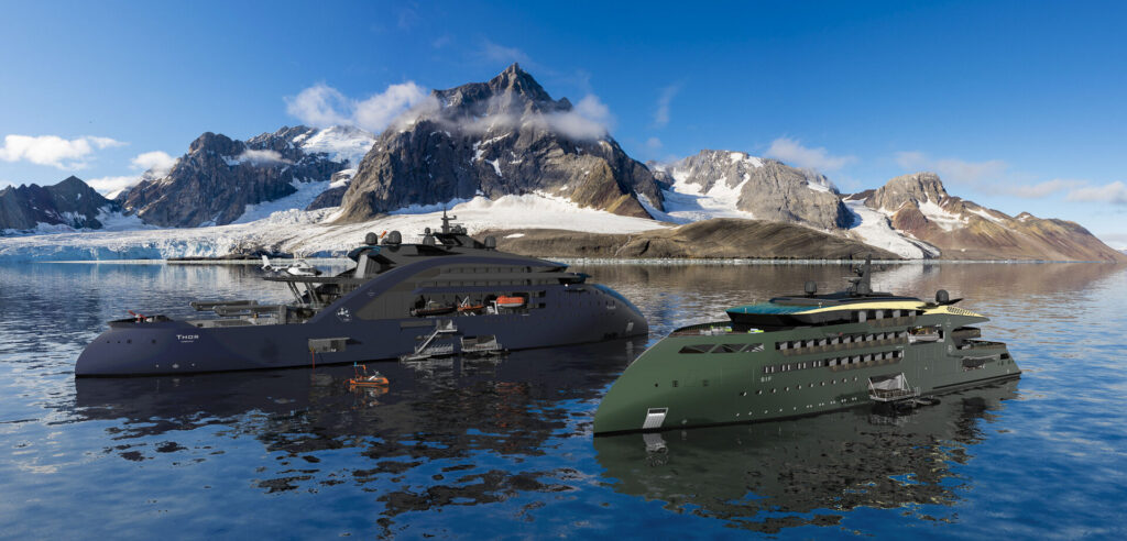
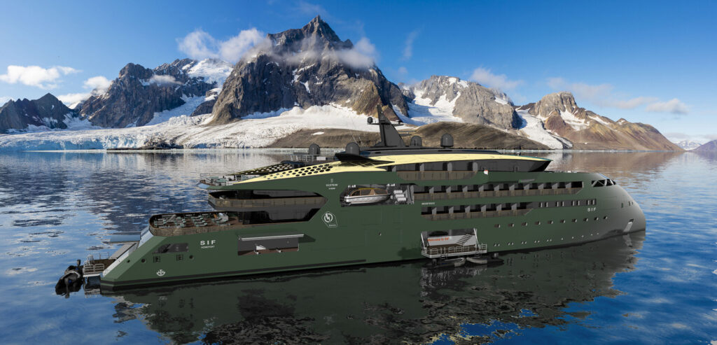
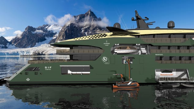
Sif electrically-powered expedition / cruise vessel (right). 
Source: Ulstein

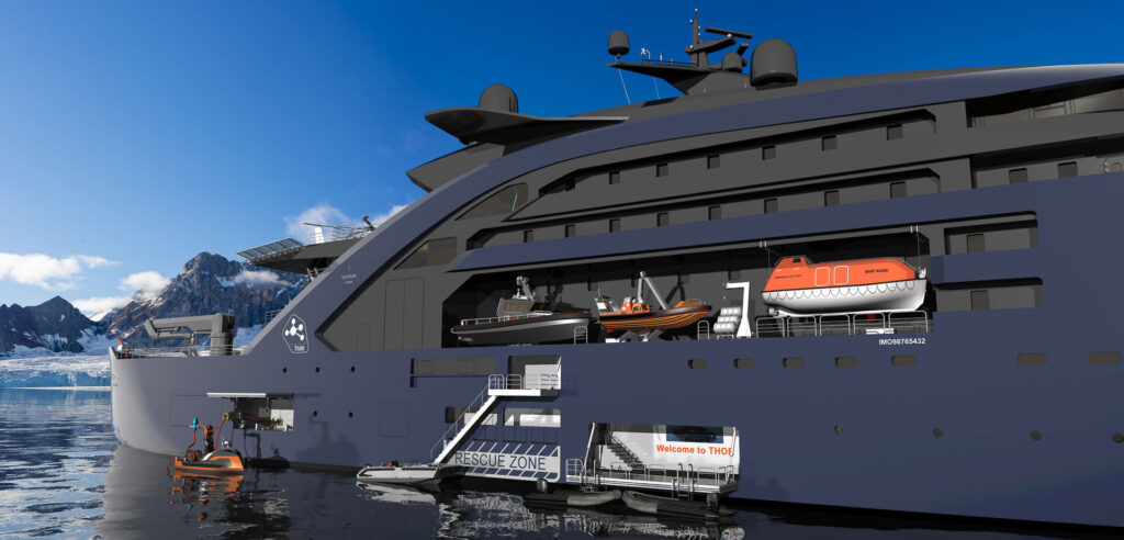
2. The MSR-powered Thor charging station

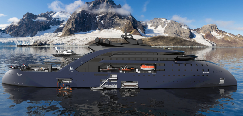
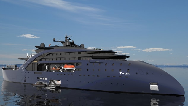
Thor is a 149-meter (500-foot) long, zero-emission, nuclear-powered vessel that features Ulstein’s striking, backwards-sloping X-bow, which is claimed to result in a smoother ride, higher speed while using less energy, and less mechanical wear than a ship with a conventional bow. 

For its R3 mission, Thor would be outfitted with work boats, cranes, a helicopter landing pad, unmanned aerial vehicles (UAVs), unmanned surface vessels, firefighting equipment, rescue booms, a lecture hall and laboratories.

As a charging station, Thor would be sized to recharge four all-electric vessels simultaneously.

Thor.  Source: Ulstein

Thor also could serve as a floating power station, replacing diesel power barges in some developing countries or in some disaster areas while the local electric power infrastructure is being repaired.

Ulstein projects that an operational Thor vessel could be launched in “10 to 15 years.” However, the development and licensing of a marine MSR is on the critical path for that schedule.  

Thor, starboard side views.  Source, both graphics: Ulstein

3. The all-electric Sif expedition / cruise ship

Sif, named after the goddess who was Thor’s wife, is a design concept for a 100-meter (330-foot) long, all-electric, zero-emission expedition / cruise ship designed to operate with minimal impact in environmentally sensitive areas. The ship will be powered by a new generation of solid batteries that are expected to offer greater capacity and resistance to fire than lithium-ion batteries used commonly today.  It will be periodically recharged at sea by Thor.

The ship can accommodate 80 passengers and 80 crew. 

Sif, starboard side view.  Source, both graphics: Ulstein

4. A marine MSR power plant

The pressurized water reactor (PWR) is the predominant marine nuclear power plant in use today, primarily in military vessels, but also in Russian icebreakers and a floating nuclear power plant in the Russian Arctic. 

Ulstein reported that it has been exploring MSR technology because of its favorable operating and safety characteristics. For example, an MSR operates at atmospheric pressure (unlike a PWR) and passive features and systems maintain safety in an emergency. If the core overheats, the molten salt fuel/coolant mixture automatically drains out of the reactor and into a containment vessel where it safely solidifies and can be reused.  You’ll find a good overview of MSR technology here: https://whatisnuclear.com/msr.html

While a few experimental MSRs have operated in the past, no MSR has been subject to a commercial nuclear licensing review, even for a land-based application. Ulstein favors a thorium-fueled MSR. The thorium-uranium-233 fuel cycle introduces additional technical and nuclear licensing uncertainties because of the lack of operational and nuclear regulatory precedents.

Several firms are developing MSR concepts. However, the combination of a marine MSR and a thorium fuel cycle remains elusive. Two uranium-fueled marine MSR design concepts are described below.

Seaborg Technologies

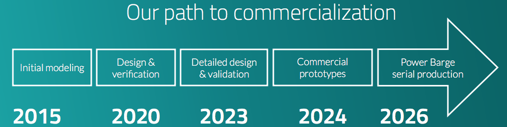
The Danish firm Seaborg Technologies (https://www.seaborg.com), founded in 2014, is developing a compact MSR (CMSR) with a rating of about 250 MWt / 100 MWe for use in power barges (floating nuclear power plants) of their own design (see my 16 May 2021 post). The thermal-spectrum CMSR uses uranium-235 fuel in a molten proprietary salt, with a separate sodium hydroxide (NaOH) moderator.  

A Seaborg Technologies CMSR module could generate 100 MWe. Dump tank shown below reactor. Source: Seaborg via NEI (2022)

Seaborg’s development time line calls for a commercial CMSR prototype to be built in 2024, with commercial production of power barges beginning in 2026. 

Source: Seaborg (2022)

In April 2022, Seaborg and the Korean shipbuilding firm Samsung Heavy Industries signed a partnership agreement for manufacturing and selling turnkey CMSR power barges. 

On 10 June 2022, Seaborg was selected by the European Innovation Council to receive a significant (potentially up to €17.5 million) innovation grant to help accelerate their work on the CMSR.

CORE-POWER and the Southern Company consortium

The UK firm CORE-POWER Ltd. (https://corepower.energy), founded in 2018, began with a concept for a compact uranium-235 fueled, molten chloride salt reactor named the m-MSR for marine applications. This modular, inherently safe, 15 MWe micro-reactor system was designed as a zero-carbon replacement power source for the fossil-fueled power plants in many existing commercial marine vessels.  It also was intended for use as the original power source for new vessels, as proposed for the Earth 300 Eco-Yacht design concept unveiled by entrepreneur Aaron Olivera in April 2021 (see my 17 April 2021 post). The power output of a modular CORE-POWER m-MSR installation could be scaled to meet operational needs by adding reactor modules in compact arrangements suitable for shipboard installation. 

A set of six small, compact CORE-POWER m-MSR modules
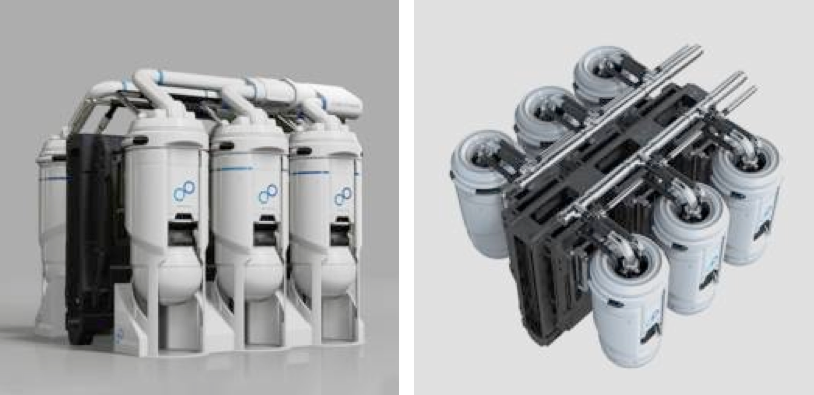
could generate 90 MWe. Dump tank not shown. Source: CORE-POWER

In November 2020, CORE-POWER announced that it had joined an international consortium to develop MSRs. This team includes the US nuclear utility company Southern Company (https://www.southerncompany.com), US small modular reactor developer TerraPower (https://www.terrapower.com) and nuclear technology company Orano USA (https://www.orano.group/usa/en). In the consortium, TerraPower is responsible for the fast-spectrum Molten Chloride Fast Reactor (MCFR). CORE-POWER is responsible for maritime readiness and regulatory approvals.

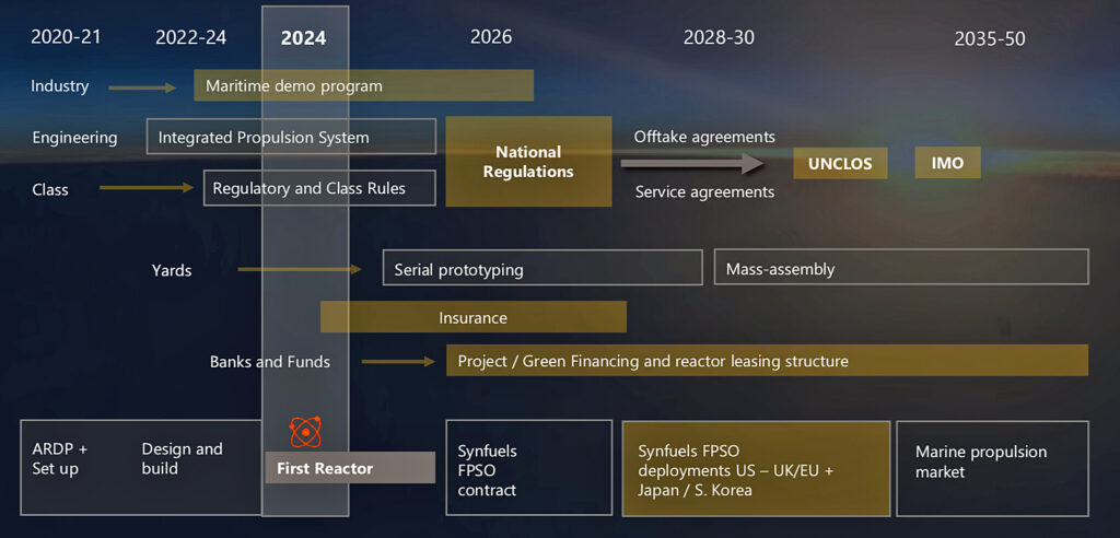
This consortium applied to the US Department of Energy (DOE) to participate in cost-share risk reduction awards under the Advanced Reactor Demonstration Program (ARDP), to develop a prototype MCFR as a proof-of-concept for a medium-scale commercial-grade reactor. In December 2020, the consortium was awarded $90.4 million, with the goal of demonstrating the first MCFR in 2024.  DOE reported, “They expect to begin testing in a $20 million integrated effects test facility starting in 2022. The team has successfully scaled up the salt manufacturing process to enable immediate testing. Data generated from the test facility will be used to validate thermal hydraulics and safety analysis codes for licensing of the reactor.”In February 2021, CORE-POWER presented the MCFR development schedule in the following chart, which shows the MCFR becoming available for deployment in marine propulsion in about 2035.  This is within the 10 to 15 year timescale projected by Ulstein for their first Thor vessel.

Source: CORE-POWER (2021)

5. In conclusion

A seaborne nuclear-powered “charging station” supporting a small fleet of all-electric marine vessels provides a zero-carbon solution for operating in protected, environmentally sensitive areas that otherwise would be off limits to visitors. Ulstein’s concept for the MSR-powered Thor R3 vessel and the Sif companion vessel is a clever approach for implementing that strategy.

It appears that a uranium-fueled marine MSR could be commercially available in the 10 to 15 year time frame Ulstein projects for deploying Thor and Sif.  The technical and nuclear regulatory uncertainties associated with a thorium-fueled marine MSR will require a considerably longer time frame. 

6. For additional information 

Ulstein Thor & Sif

Video

Seaborg CMSR

CORE-POWER m-MSR

Blue Glaciers, Blue Icebergs and the Antarctic Museum of Modern Art

Peter Lobner, 1 September 2020

Why is glacial ice blue?

The US Geologic Survey (USGS) provides a basic explanation of why glacial ice is blue:

“The red-to-yellow (longer wavelength) parts of the visible spectrum are absorbed by ice more effectively than the blue (shorter wavelength) end of the spectrum. The longer the path light travels in ice, the more blue it appears.  This is because the other colors are being preferentially absorbed and make up an ever smaller fraction of the light being transmitted and scattered through the ice.”

Blue ice with natural lighting inside a glacial ice cave, Grindelwald, Switzerland.
Source: P. Lobner photo

The key to blue ice is selective absorption, which occurs in a special kind of ice that is produced on land with the help of pressure and time.  Becky Oskin provides the following general insights into how this process occurs in her 2015 article, “Why Are Some Glaciers Blue?”

  1. When glacial ice first freezes, it is filled with air bubbles that are effective in scattering light passing through the ice. As that ice gets buried and compressed by subsequent layers of younger ice, the air bubbles become smaller and smaller.  With less scattering of light by the air bubbles, light can penetrate more deeply into the ice and the older ice starts to take on a blue tinge. Blue ice is old ice.
  2. Patches of blue-hued ice emerge on the surface of glaciers where wind and sublimation have scoured old glaciers clean of snow and young ice. 
  3. Blue ice also may emerge at the edges of a glacial icepack, where fragments of glaciers tumble into the sea and reveal a fresh edge of the old ice.

Stephen Warren’s 2019 paper, “Optical properties of ice and snow,” provides the following more technical description of the selective absorption process in ice:

  1. “Ice is a weak filter for red light..….the absorption coefficient of ice increases with wavelength from blue to red (but the absorption spectrum is quite complex). The absorption length…… is approximately 2 meters at (a wavelength of ) λ = 700 nm (nanometers, red end of the visible spectrum) but approximately 200 meters at λ = 400 nm (blue-violet end of the visible spectrum). Photons at all wavelengths of visible light will survive without absorption, and be reflected or transmitted, unless the path length through ice is long enough to significantly absorb the red light.”…..”Ice develops a noticeable blue color in glacier crevasses and in icebergs, especially in marine ice (i.e., icebergs calved from glacial ice shelves), because of its lack of (air) bubbles (which would otherwise cause scattering and limit light transmission through the ice).”
  2. The absorption length is the distance into a material where the beam flux has dropped to 1/e (1/2.71828 = 0.368 = 37%) of its incident flux.  For light at the red end of the spectrum, that is a relatively short distance of about 2 meters.  This means that, in 2 meters, absorption decreases the red light component of beam flux by a factor of 1/e to about 37% of the original incident red light.  In another 2 meters, the red light beam flux is reduced to about 14% of the original incident red light. At the same distances, the blue-violet end of the spectrum has hardly been attenuated at all. 

You can see that even modest size pieces of glacial ice (several meters in length / diameter) should be able to attenuate the red-to-yellow end of the spectrum and appear with varying degrees of blue tints. Looking into an ice borehole in an Antarctic ice sheet shows how intensely blue the deeper part of the glacial ice appears to the viewer on the surface.  The removed ice core is a slender cylinder of ice that looks like clear ice when viewed from the side. 

Looking down into an Antarctic ice borehole.
Source: https://giglinthefield.wordpress.com/tag/antarctica/
A segment of an ice core sample.
Source: https://sites.google.com/site/amblerspsychrophiles/

So… why is snow white? Light does not penetrate into snow very far before being scattered back to the viewer by the many facets of uncompressed snow on the surface.  Thus, there is almost no opportunity for light absorption by the snow, and hence very little selective absorption of the red-to-yellow part of the visible spectrum.

For the same reason, sea ice, which is formed by the seasonal freezing of the sea surface, appears white because of the high concentration of entrained air bubbles (relative to glacial ice) that causes rapid scattering of incident light.  Sea ice does not go through the metamorphism that produces glacial ice on land.

What is glacial ice?

The USGS describes glacial ice as follows:  “Glacier ice is actually a mono-mineralic rock (a rock made of only one mineral, like limestone which is composed of the mineral calcite). The mineral ice is the crystalline form of water (H2O). It forms through the metamorphism of tens of thousands of individual snowflakes into crystals of glacier ice. Each snowflake is a single, six-sided (hexagonal) crystal with a central core and six projecting arms. The metamorphism process is driven by the weight of overlying snow. During metamorphism, hundreds, if not thousands of individual snowflakes recrystallize into much larger and denser individual ice crystals. Some of the largest ice crystals observed at Alaska’s Mendenhall Glacier are nearly one foot in length.”

A small chunk of clear glacial ice retrieved from Pléneau Bay, Antarctica.
Source: P. Lobner photo

Where do glaciers exist?

The National Snow and Ice Data Center (NSIDC) reports that, “glaciers occupy about 10 percent of the world’s total land area, with most located in polar regions like Antarctica, Greenland, and the Canadian Arctic. Glaciers can be thought of as remnants from the last Ice Age, when ice covered nearly 32 percent of the land, and 30 percent of the oceans. Most glaciers lie within mountain ranges that show evidence of a much greater extent during the ice ages of the past two million years, and more recent indications of retreat in the past few centuries.”

Glaciers exist on every continent except Australia. The approximate distribution of glaciers is:

  1. 91% in Antarctica
  2. 8% in Greenland
  3. Less than 0.5% in North America (about 0.1% in Alaska)
  4. 0.2% in Asia
  5. Less than 0.1% is in South America, Europe, Africa, New Zealand, and New Guinea (Irian Jaya).

There are several schemes for classifying glaciers; some are described in the references at the end of this article.  For simplicity, let’s consider two basic types.

  1. polar glacier is defined as one that is below the freezing temperature throughout its mass for the entire year.  Polar glaciers exist in Antarctica and Greenland as continental scale ice sheets and smaller scale ice caps and ice fields.
  2. temperate glacier is a glacier that’s essentially at the melting point, so liquid water coexists with glacier ice. A small change in temperature can have a major impact on temperate glacier melting, area, and volume. Glaciers not in Antarctica or Greenland are temperate glaciers.  In addition, some of the glaciers on the Antarctic Peninsula and some of Greenland’s southern outlet glaciers are temperate glaciers.

How old is glacier ice?

Some glacial ice is extremely old, while in many areas of the world, it is much younger than you might have expected.

USGS reports:  “Parts of the Antarctic Continent have had continuous glacier cover for perhaps as long as 20 million years. Other areas, such as valley glaciers of the Antarctic Peninsula and glaciers of the Transantarctic Mountains may date from the early Pleistocene (starting about 2.6 million years ago and lasting until about 11,700 years ago). For Greenland, ice cores and related data suggest that all of southern Greenland and most of northern Greenland were ice-free during the last interglacial period, approximately 125,000 years ago. Then, climate (in Greenland) was as much as 3-5o F warmer than the interglacial period we currently live in.”

“Although the higher mountains of Alaska have hosted glaciers for as much as the past 4 million years, most of Alaska temperate glaciers are generally much, much younger. Many formed as recently as the start of the Little Ice Age, approximately 1,000 years ago. Others may date from other post-Pleistocene (younger than 11,700 years ago) colder climate events.”

  1. The age of the oldest glacier ice in Antarctica may approach 20,000,000 years old.
  2. The age of the oldest glacier ice in Greenland may be more than 100,000 years old, but less than 125,000 years old.
  3. The age of the oldest Alaskan glacier ice ever recovered was about 30,000 years old.

Blue glacial ice along the coast of the West Antarctic Peninsula

In February 2020, my wife and I made a well-timed visit to the West Antarctic Peninsula.  One particularly amazing spot was Pléneau Bay, which easily could earn the title “Antarctic Museum of Modern Art” because of the many fanciful iceberg shapes floating gently in this quiet bay.  Following is a short photo essay highlighting several of the beautiful blue glacial ice features we saw on this trip.

Small blue iceberg in the Lemaire Channel. Source: P. Lobner photo
Zodiacs in what could be called the “Antarctic Museum of Modern Art”
 in Pléneau Bay. Source: J. Lobner photo
Crabeater seal amid the blue icebergs in Pléneau Bay. 
Source: J. Lobner photo
Exotic blue iceberg shapes in Pléneau Bay. Source: P. Lobner photo
The tall, fluted wall of a large blue iceberg in Pléneau Bay.
Source: J. Lobner photo
A chunk of faceted glacial ice among the brash sea ice in Hanusse Bay / Crystal Sound. Source: P. Lobner photo
Blue icebergs among the brash sea ice at Prospect Point
(above & below). Source: P. Lobner photos
A humpback whale resting among the blue icebergs in Cierva Cove (above) and diving (below). Source: P. Lobner photos
This iceberg (above & below) in Cierva Cove looks like a majestic blue sailing ship. 
Source: P. Lobner photos
Another exotic blue iceberg in Cierva Cove. Source: J. Lobner photo
Zodiac among blue icebergs in Cierva Cove. Source: P. Lobner photo
The large underwater part of this iceberg radiates blue in Cierva Cove.
Source: P. Lobner photo
A sea cave provides a view into the blue ice underlying an ice shelf.
Source: P. Lobner photo

Examples of blue glacial ice in Switzerland & New Zealand 

In previous years, my wife and I visited a temperate glacier and ice cave in Grindelwald, Switzerland and hiked on the temperate Franz Josef Glacier on the South Island of New Zealand.  Following is a short photo essay that should give you an idea of the complex terrain of these glaciers and the smaller scale blue ice features visible on the surface.  In contrast, the ice cave was a unique, immersive, very blue experience.  The blue color inside the cave looked like the eerie blue light from Cherenkov radiation, like you’d see in an operating pool-type nuclear research reactor.

Inside a glacial ice cave in Grindelwald, Switzerland.
Source: P. Lobner photo
Franz Joseph Glacier showing a general blue tint in some surface ice (above) and more intense blue in smaller areas (below), South Island, 
New Zealand.  Source:  P. Lobner photos
Franz Joseph Glacier details (above & below). 
Source: P. Lobner photos

For more information:

  1. “What is a glacier?” US Geologic Survey (USGS) website:  https://www.usgs.gov/faqs/what-a-glacier?qt-news_science_products=0#qt-news_science_products
  2.  “Why Glacier Ice is Blue,” USGS website: https://www.usgs.gov/faqs/why-glacier-ice-blue?qt-news_science_products=0#qt-news_science_products
  3.  “Common Questions and Myths About Glaciers,” National Park Service (NPS) website: https://www.nps.gov/glba/learn/nature/common-questions-and-myths-about-glaciers.htm
  4. Becky Oskin, “Why Are Some Glaciers Blue?” LiveScience website: https://www.livescience.com/51019-why-is-antarctica-ice-blue.html
  5. Stephen Warren, “Optical properties of ice and snow,” Philosophical Transactions of the Royal Society, 15 April 2019: https://royalsocietypublishing.org/doi/full/10.1098/rsta.2018.0161
  6.  “About Glaciers,” National Snow and Ice Data Center (NSIDC) website: https://nsidc.org/cryosphere/glaciers/information.html
  7. Robin George Andrews, “Icebergs can be emerald green. Now we know why,” National Geographic, 15 March 2019: https://www.nationalgeographic.com/science/2019/03/icebergs-can-be-emerald-green-now-we-know-why

Antarctica – What’s Under All That Ice?

Peter Lobner, Updated 24 August 2021

From space, Antarctica gives the appearance of a large, ice-covered continental land mass surrounded by the Southern Ocean.  The satellite photo mosaic, below, reinforces that illusion.  Very little ice-free rock is visible, and it’s hard to distinguish between the continental ice sheet and ice shelves that extend into the sea.

Satellite mosaic image of Antarctica created by Dave Pape, 
adapted to the same orientation as the following maps. 
 Source.  https://geology.com/world/antarctica-satellite-image.shtml

The following topographical map presents the surface of Antarctica in more detail, and shows the many ice shelves (in grey) that extend beyond the actual coastline and into the sea.  The surface contour lines on the map are at 500 meter (1,640 ft) intervals.

Map of Antarctica and the Southern Ocean showing the topography of Antarctica (as blue lines), research stations of the United States and the United Kingdom (in red text), ice-free rock areas (in brown), ice shelves (in gray) and names of the major ocean water bodies (in blue uppercase text).
Source: LIMA Project (Landsat Image Mosaic of Antarctica) via Wikipedia

The highest elevation of the ice sheet is 4,093 m (13,428 ft) at Dome Argus (aka Dome A), which is located in the East Antarctic Ice Sheet, about 1,200 kilometers (746 miles) inland.  The highest land elevation in Antarctica is Mount Vinson, which reaches 4,892 meters (16,050 ft) on the north part of a larger mountain range known as Vinson Massif, near the base of the Antarctic Peninsula.  This topographical map does not provide information on the continental bed that underlies the massive ice sheets.

A look at the bedrock under the ice sheets: Bedmap2 and BedMachine

In 2001, the British Antarctic Survey (BAS) released a topographical map of the bedrock that underlies the Antarctic ice sheets and the coastal seabed derived from data collected by international consortia of scientists since the 1950s. The resulting dataset was called  BEDMAP1.  

In a 2013 paper, P. Fretwell, et al. (a very big team of co-authors), published the paper, “Bedmap2: Improved ice bed, surface and thickness datasets for Antarctica,” which included the following bed elevation map, with bed elevations color coded as indicated in the scale on the left.  As you can see, large portions of the Antarctic “continental” bedrock are below sea level.

Bedmap2 bed elevation grid.  Source:  Fretwell 2013, Fig. 9

You can read the 2013 Fretwell paper here:  https://www.the-cryosphere.net/7/375/2013/tc-7-375-2013.pdf

For an introduction to Antarctic ice sheet thickness, ice flows, and the topography of the underlying bedrock, please watch the following short (1:51) 2013 video, “Antarctic Bedrock,” by the National Aeronautics and Space Administration’s (NASA’s) Scientific Visualization Studio:

NASA explained:

  • “In 2013, BAS released an update of the topographic dataset called BEDMAP2 that incorporates twenty-five million measurements taken over the past two decades from the ground, air and space.”
  • “The topography of the bedrock under the Antarctic Ice Sheet is critical to understanding the dynamic motion of the ice sheet, its thickness and its influence on the surrounding ocean and global climate. This visualization compares the new BEDMAP2 dataset, released in 2013, to the original BEDMAP1 dataset, released in 2001, showing the improvements in resolution and coverage.  This visualization highlights the contribution that NASA’s mission Operation IceBridge made to this important dataset.”

On 12 December 2019, a University of California Irvine (UCI)-led team of glaciologists unveiled the most accurate portrait yet of the contours of the land beneath Antarctica’s ice sheet.  The new topographic map, named “BedMachine Antarctica,”  is shown below.

BedMachine Antarctica topographical map showing the underlying ground features and the large portions of the continental bed that are below sea level.  
 Credit: Mathieu Morlighem / UCI

UCI reported:

  • “The new Antarctic bed topography product was constructed using ice thickness data from 19 different research institutes dating back to 1967, encompassing nearly a million line-miles of radar soundings. In addition, BedMachine’s creators utilized ice shelf bathymetry measurements from NASA’s Operation IceBridge campaigns, as well as ice flow velocity and seismic information, where available. Some of this same data has been employed in other topography mapping projects, yielding similar results when viewed broadly.”
  • “By basing its results on ice surface velocity in addition to ice thickness data from radar soundings, BedMachine is able to present a more accurate, high-resolution depiction of the bed topography. This methodology has been successfully employed in Greenland in recent years, transforming cryosphere researchers’ understanding of ice dynamics, ocean circulation and the mechanisms of glacier retreat.”
  • “BedMachine relies on the fundamental physics-based method of mass conservation to discern what lies between the radar sounding lines, utilizing highly detailed information on ice flow motion that dictates how ice moves around the varied contours of the bed.”

The net result is a much higher resolution topographical map of the bedrock that underlies the Antarctic ice sheets.  The authors note:“This transformative description of bed topography redefines the high- and lower-risk sectors for rapid sea level rise from Antarctica; it will also significantly impact model projections of sea level rise from Antarctica in the coming centuries.”

You can take a visual tour of BedMachine’s high-precision model of Antarctic’s ice bed topography here.  Enjoy your trip.

There is significant geothermal heating under parts of Antarctica’s bedrock

West Antarctica and the Antarctic Peninsula form a connected rift / fault zone that includes about 60 active and semi-active volcanoes, which are shown as red dots in the following map.  

Volcanoes located along the branching West Antarctic Fault/Rift System.
Source:  James Kamis, Plate Climatology, 4 July 2017

In a 29 June 2018 article on the Plate Climatology website, author James Kamis presents evidence that the fault / rift system underlying West Antarctica generates a significant geothermal heat flow into the bedrock and is the source of volcanic eruptions and sub-glacial volcanic activity in the region.  The heat flow into the bedrock and the observed volcanic activity both contribute to the glacial melting observed in the region.  You can read this article here:

http://www.plateclimatology.com/geologic-forces-fueling-west-antarcticas-larsen-ice-shelf-cracks/

The correlation between the locations of the West Antarctic volcanoes and the regions of higher heat flux within the fault / rift system are evident in the following map, which was developed in 2017 by a multi-national team.

Geothermal heat flux distribution at the ice-rock interface superimposed on subglacial topography.  Source:  Martos, et al., Geophysical Research Letter 10.1002/2017GL075609, 30 Nov 2017

The authors note: “Direct observations of heat flux are difficult to obtain in Antarctica, and until now continent-wide heat flux maps have only been derived from low-resolution satellite magnetic and seismological data. We present a high-resolution heat flux map and associated uncertainty derived from spectral analysis of the most advanced continental compilation of airborne magnetic data. …. Our high-resolution heat flux map and its uncertainty distribution provide an important new boundary condition to be used in studies on future subglacial hydrology, ice sheet dynamics, and sea level change.”  This Geophysical Research Letter is available here:  

https://agupubs.onlinelibrary.wiley.com/doi/pdf/10.1002/2017GL075609

The results of six Antarctic heat flux models developed from 2004 to 2017 were compared by Brice Van Liefferinge in his 2018 PhD thesis.  His results, shown below, are presented on the Cryosphere Sciences website of the European Sciences Union (EGU). 

Spatial distributions of geothermal heat flux: (A) Pollard et al. (2005) constant values, (B) Shapiro and Ritzwoller (2004): seismic model, (C) Fox Maule et al. (2005): magnetic measurements, (D) Purucker (2013): magnetic measurements, (E) An et al. (2015): seismic model and (F) Martos et al. (2017): high resolution magnetic measurements.  Source:  Brice Van Liefferinge (2018) PhD Thesis.

Regarding his comparison of Antarctic heat flux models, Van Liefferinge reported:  

  • “As a result, we know that the geology determines the magnitude of the geothermal heat flux and the geology is not homogeneous underneath the Antarctic Ice Sheet:  West Antarctica and East Antarctica are significantly distinct in their crustal rock formation processes and ages.”
  • “To sum up, although all geothermal heat flux data sets agree on continent scales (with higher values under the West Antarctic ice sheet and lower values under East Antarctica), there is a lot of variability in the predicted geothermal heat flux from one data set to the next on smaller scales. A lot of work remains to be done …” 

The effects of geothermal heating are particularly noticeable at Deception Island, which is part of a collapsed and still active volcanic crater near the tip of the Antarctic Peninsula.  This high heat flow volcano is in the same major fault zone as the rapidly melting / breaking-up Larsen Ice Shelf.  The following map shows the faults and volcanoes in this region.  

Key geological features in the Larsen “C” sea ice segment area.  
Source:  James Kamis, Plate Climatology, 4 July 2017
Tourists enjoying the geothermally heated ocean water at Deception Island.  
Source: Public domain

So, if you take a cruise to Antarctica and the Cruise Director offers a “polar bear” plunge, I suggest that you wait until the ship arrives at Deception Island.  Remember, this warm water is not due to climate change.  You’re in a volcano.

For more information on Bedmap 2 and BedMachine:

  • “Antarctic Bedrock,” Visualizations by Cindy Starr,  NASA Scientific Visualization Studio, Released on June 4, 2013:  https://svs.gsfc.nasa.gov/4060
  • Morlighem, M., Rignot, E., Binder, T. et al. “Deep glacial troughs and stabilizing ridges unveiled beneath the margins of the Antarctic ice sheet,” Nature Geoscience (2019) doi:10.1038/s41561-019-0510-8:  https://www.nature.com/articles/s41561-019-0510-8

More information on geothermal heating in the West Antarctic rift / fault zone:

200th Anniversary of the Discovery of Antarctica: 28 January 2020

Peter Lobner

During his second voyage in 1773, British Captain James Cook became the first to cross the Antarctic Circle, but he was turned back by heavy sea ice without ever sighting the coast of Antarctica.  It took 47 years before a Russian expedition, led by Estonian Fabien von Bellingshausen, sighted the coast of Antarctica. As the expedition leader, Bellingshausen generally is credited with the discovery of Antarctica on 28 January 1820.  Just two days later, on 30 January 1820, a British expedition to the South Shetland Islands, led by Irish Lieutenant Edward Bransfield, sighted the tip of the Antarctic Peninsula.  Bransfield is credited by some with the discovery of Antarctica.  In this post, we’ll take a look at the voyages of these three pioneering Antarctic explorers.


Map of Antarctica and the Southern Ocean showing the topography of Antarctica (as blue lines), research stations of the United States and the United Kingdom (in red text), ice-free rock areas (in brown), ice shelves (in gray) and names of the major ocean water bodies (in blue uppercase text).  Source: adapted from LIMA Project (Landsat Image Mosaic of Antarctica) via Wikipedia

Captain James Cook  – First crossing of the Antarctic Circle,  17 January 1773

Setting out on their second voyage from England in July 1772, Captain James Cook (1728-1779) and his crew, on His Majesty’s Ship Resolution, circumnavigated the globe travelling as far south as possible to determine whether there actually was a great southern continent.  The route covered during this voyage is shown in the following map.

Route of James Cook’s second voyage.  Source:  Jon Platek via Wikipedia

On 17 January 1773, Cook made the first recorded crossing of the Antarctic Circle, which he reported in his log:

“At about a quarter  past 11 o’clock we cross’d the Antarctic Circle, for at Noon we were by observation four miles and a half south of it and are undoubtedly the first and only ship that ever cross’d that line.”

Cook crossed the Antarctic Circle three times during his second voyage.  The last crossing, on 30 January 1773, was to be the most southerly penetration of Antarctic waters, reaching latitude 71°10’ S, longitude 106°54’ W.  The ship was forced back due to solid sea ice.  Cook came within about 240 km (150 mi) of the Antarctic mainland on his second voyage.

Cook’s southernmost approach to Antarctica (yellow pin, left).  Source:  Google Earth

Fabien von Bellingshausen – First sighting of Antarctica, 28 January 1820

In 1818, the Russian Empire, ruled by Czar Alexander I, organized two expeditions to study the polar regions, one for mapping the Arctic and one for sailing further south than Captain James Cook’s second voyage 45 years earlier.  The southern polar expedition was led by the prominent cartographer Fabien Gottlieb Benjamin von Bellingshausen, who was born in 1778 on Saaremaa, the largest island in today’s Republic of Estonia.  This was to became known as the Bellingshausen Expedition. 

The expedition consisted of two ships, Bellingshausen’s 985 ton flagship sloop Vostok, and the 530 ton support sloop Mirnyi, under the command of Mikhail Lazarev (Bellingshausen’s second-in-command).  An exhibit at the Estonian Maritime Museum in Tallinn reported:  “The largest proportion (a whopping 65.8 tons) of the food stock on the Bellingshausen expedition consisted of wheat and rye cookies.  In addition, they brought 28 tons of salted meat and 20.5 tons of dried peas.  In ports, the crew also acquired cereal and fresh food.”  In Antarctic waters, icebergs would supply their fresh water needs.

On 4 June 1819, the expedition departed from the Russian naval island base at Kronstadt, just off the coast from Saint Petersburg. Seven months later, the expedition crossed the Antarctic Circle on 26 January 1820.

The Bellingshausen expedition is credited with being the first to reach Antarctica on 28 January 1820, when the two ships approached to within 20 miles (32 km) of the Antarctic coast, at latitude 69°21’28” S, longitude 2°14’50” W,  in an area now known as Princess Martha Coast in East Antarctica.  Bellingshausen reported sighting an ice shelf that today is known as the Fimbul ice shelf.

Location of Bellingshausen’s first sighting of Antarctica on 28 January 1820 
(yellow pin, upper right).  Source:  Google Earth

Bellingshausen did not claim to have discovered Antarctica, but his descriptions of what he saw agree very well with what the Princess Martha Coast is now known to look like.  On the basis of this sighting and the coordinates given in his log book, Bellingshausen generally is credited (e.g., the British polar historian A. G. E. Jones) with the discovery of  the Antarctic continent.

In their subsequent circumnavigation of the Antarctic continent, Bellingshausen and Lazarev became the first explorers to see and officially discover several parts of the Antarctic landmass.   On 22 February 1820, the Vostok and Mirnyi were hit by the worst storm of the voyage and were forced to sail north, arriving in Sydney, Australia in April.  After several months exploring the South Pacific and then hearing about the sighting of Antarctica by the British (Edward Bransfield and William Smith), the Bellingshausen Expedition sailed from Sydney on 11 November 1820 to continue exploring the Antarctic. On 24 December 1820, the two ships once again were south of the Antarctic Circle.  On this part of the voyage, Bellingshausen discovered and named Peter I Island and the Alexander Coast, now known as Alexander Island, along the west coast of the Antarctic Peninsula.

The circumnavigation route followed by the Bellingshausen Expedition is shown in the following map.  Bellingshausen became only the second explorer, after Cook, to have circumnavigated Antarctica.

Route map of the Bellingshausen Expedition to Antarctica: 1819-21.
Source:  Bourrichon via Wikipedia

The Bellingshausen expedition returned to Kronstadt on 4 August 1821, ending a voyage that had lasted two years and 21 days and covered about 50,000 miles (80,467 km).  After his return, Bellingshausen was promoted to the rank of Admiral and Lazarev was promoted to the rank of Lieutenant–Captain.  His travel account was not published until ten years later.

As part of the International Geophysical Year (IGY) in the mid-1950s, the Soviet Union established its first two Antarctic bases, which were named Mirnyi (established 13 February 1956) and Vostok (established 6 December 1957), in honor of the ships in the Bellingshausen Expedition.

2003 Estonian stamp commemorating Bellingshausen’s 
discovery of Antarctica.  Source: eBay

The Bellingshausen expedition was commemorated on a 2003 Estonian stamp that features a portrait of Bellingshausen and a drawing of his flagship Vostok over a map showing the route of his Antarctic expedition.

Edward Bransfield – Sighting of Antarctica, 30 January 1820

In February 1819, British merchant ship owner William Smith, aboard his vessel The Williams, was sailing from Buenos Aires, Argentina to Valparaiso, Chile.   To catch the prevailing winds, he sailed unusually far south of Cape Horn and, on 19 February 1819, sighted previously unknown islands in the Southern Ocean.  To confirm his sighting and to chart the islands, Royal Navy officials in Valpariso chartered his ship and assigned Sailing Master Lieutenant Edward Bransfield, from Ballinacurra, Ireland (near Cork), to accompany Smith on an expedition back to the islands, which would become known as the South Shetland Islands.  During this expedition,  Bransfield landed on King George Island and took formal possession on behalf of King George III.  

On 30 January 1820, Bransfield sighted the Trinity Peninsula, which is the northernmost tip of the Antarctic Peninsula.  His sighting was made at about latitude 63°50’S and longitude 60°30’W.

Location of Bransfield’s first sighting of Antarctica (yellow pin, top center) on 30 January 1820.  Source:  Google Earth

After the initial sighting, Bransfield charted a segment of the Trinity Peninsula and followed the edge of the ice sheet in a north-easterly direction, where he discovered various points on Elephant Island and Clarence Island, which he formally claimed for the British Crown. In his log, Bransfield made a note of two “high mountains, covered with snow”, one of which subsequently was named Mount Bransfield in his honor.  The Bransfield Strait between the South Shetland Islands and the Antarctic Peninsula also was named in his honor in 1822 by Antarctic explorer James Weddell. 

Bransfield’s track in Antarctic.  Source:  Edited version by Jim Wilson, http://rememberingedwardbransfield.ie/voyage-of-discovery/

Since Bransfield’s sighting, the tip of the Antarctic Peninsula has been known variously as Trinity Land, Palmer Land, Graham Land, and Land of Louis Philippe.  Prime Head is the northernmost point of this peninsula. 

Bransfield’s expedition charts were given to the Admirality and currently are in the possession of the UK Hydrographic department in Taunton, Somerset.

In 2000, Bransfield’s historic achievement was recognized when the Royal Mail issued a stamp in his honor. Since no likeness of the man survives, the stamp depicted an image of the RRS Bransfield, a British Antarctic surveying vessel.

2000 Royal Mail commemorative stamp. 
Source: Commonwealth Stamps Opinion

To commemorate the 200th anniversary of Edward Bransfield’s sighting of Antarctica (and some say, his discovery of Antarctica), a memorial by sculptor Matt Thompson will be erected in Ballinacurra, Ireland in January 2020.

Edward Bransfield memorial, work in progress.
Source: Tony Whelan photo, Afloat.ie

Estonia’s Antarktika 200 expedition

To commemorate the 200th anniversary of the discovery of Antarctica by the Bellingshausen Expedition, the Estonian Maritime Museum and NGO Thetis Expeditions have organized a scientific expedition from Kronstadt, Russia to the Antarctic peninsula by a crew of 12 aboard the 24 meter, 95 ton, Estonian-registered sailing yacht S/Y Admiral Bellingshausen.

S/Y Admiral Bellingshausen.
Source: maritimetraffic.com

The planned route, which includes about 50 stops, and approximately follows the Bellingshausen’s route to and from the Southern Ocean, is shown in the following map.  The crew will take samples of pollen, water and microplastics while on the voyage, for researchers at Estonia’s University of Tartu.  The expedition includes food of Estonian origin to the largest possible extent, and probably a better selection of food than on Bellingshausen’s 1819 – 1821 voyage.

Antarktika 200 route map.  Source: International Maritime Rescue Federation

The ship departed Tallinn harbor on 14 July 2019, and headed for its first port of call at the historic Russian naval island base at Kronstadt, which was the starting point for the Bellingshausen Expedition.  

You can follow the current position on the S/Y Admiral Bellingham at the following link:

https://www.marinetraffic.com/en/ais/details/ships/shipid:5929279

On 3 January 2020, the ship was moored in Ushuaia, Argentina, in preparation for its voyage across the Drake Passage to Antarctica.  The ship is scheduled to reach Antarctica in time to celebrate the 200th anniversary of Bellingshausen’s discovery on 28 January 2020.

This voyage will be the subject of a TV documentary.  For more information on the Antarktika 200 expedition, visit the following website:

https://www.international-maritime-rescue.org/news/the-estonian-maritime-expedition-to-celebrate-the-discovery-of-antarctica-200-years-ago

Best wishes to the crew of S/Y Admiral Bellingshausen for a safe and successful voyage.

Composite map of early expeditions in Antarctic waters

The following map provides a good overview of the routes taken by the early Antarctic explorers, none of whom went ashore.  

Source: Antarctic Logistics

The first landings in Antarctica

An unconfirmed first landing at Hughes Bay, on the northwest coast of the Antarctic Peninsula, may have been made on 7 February 1821 by Captain John Davis and crew members from the American sealing ship Cecilia, which had been sailing in the vicinity of the South Shetland Islands in search of seals. The ship’s log recorded that men were ashore to look for seals at latitude 64°01’S.  The logbook entry concluded with the statement, “I think this Southern Land to be a Continent.”

The first substantiated landing in Antarctica was not made until 74 years later, on 24 January 1895, when seven men from the Norwegian whaling and sealing ship Antarctic, came ashore in the vicinity of Cape Adare, on the Ross Sea almost due south of New Zealand.  New Zealander Alexander Francis Henry von Tunzelmann is sometimes credited as being the first person to set foot on the Antarctic mainland.

For more information on Fabien Bellingshausen & Mikhail Lazarev

Fabien Gottlieb Von Bellingshausen (1778-1852):  https://antarctic-logistics.com/2010/08/28/fabian-gottlieb-von-bellingshausen/

Mikhail Lazarev (1788-1851):  https://antarctic-logistics.com/2010/08/28/mikhail-lazarev/

For more information on Edward Bransfield:

Remembering Edward Bransfield:  http://rememberingedwardbransfield.ie

NOAA’s Monthly Climate Summaries are Worth Your Attention

Peter Lobner

The National Oceanic and Atmospheric Administration’s (NOAA’s) National Centers for Environmental Information (NCEI) are responsible for “preserving, monitoring, assessing, and providing public access to the Nation’s treasure of climate and historical weather data and information.”  The main NOAA / NCEI website is here:

https://www.ncdc.noaa.gov

The “State of the Climate” is a collection of monthly summaries recapping climate-related occurrences on both a global and national scale.  Your starting point for accessing this collection is here:

https://www.ncdc.noaa.gov/sotc/

The following monthly summaries are available.

I’d like to direct your attention to two particularly impressive monthly summaries:

  • Global Summary Information, which provides a comprehensive top-level view, including the Sea Ice Index
  • Global Climate Report, which provides more information on temperature and precipitation, but excludes the Sea Ice Index information

Here are some of the graphics from the Global Climate Report for June 2019.

Source: NOAA NCEI
Source: NOAA NCEI

NOAA offered the following synopsis of the global climate for June 2019.

  • The month of June was characterized by warmer-than-average temperatures across much of the world. The most notable warm June 2019 temperature departures from average were observed across central and eastern Europe, northern Russia, northeastern Canada, and southern parts of South America.
  • Averaged as a whole, the June 2019 global land and ocean temperature departure from average was the highest for June since global records began in 1880.
  • Nine of the 10 warmest Junes have occurred since 2010.

For more details, see the online June 2019 Global Climate Reportat the following link:

https://www.ncdc.noaa.gov/sotc/global/201906

A complementary NOAA climate data resource is the National Snow & Ice Data Center’s (NSIDC’s) Sea Ice Index, which provides monthly and daily quick looks at Arctic-wide and Antarctic-wide changes in sea ice. It is a source for consistently processed ice extent and concentration images and data values since 1979. Maps show sea ice extent with an outline of the 30-year (1981-2010) median extent for the corresponding month or day. Other maps show sea ice concentration and anomalies and trends in concentration.  In addition, there are several tools you can use on this website to animate a series of monthly images or to compare anomalies or trends.  You’ll find the Sea Ice Index here:

https://nsidc.org/data/seaice_index/

The Arctic sea ice extent for June 2019 and the latest daily results for 23 July 2019 are shown in the following graphics, which show the rapid shrinkage of the ice pack during the Arctic summer.  NOAA reported that the June 2019 Arctic sea ice extent was 10.5% below the 30-year (1981 – 2010) average.  This is the second smallest June Arctic sea ice extent since satellite records began in 1979.

Source:  NOAA NSIDC
Source:  NOAA NSIDC

The monthly Antarctic results for June 2019 and the latest daily results for 23 July 2019 are shown in the following graphics, which show the growth of the Antarctic ice pack during the southern winter season. NOAA reported that the June 2019 Antarctic sea ice extent was 8.5% below the 30-year (1981 – 2010) average.  This is the smallest June Antarctic sea ice extent on record.

Source:  NOAA NSIDC
Source:  NOAA NSIDC

I hope you enjoy exploring NOAA’s “State of the Climate” collection of monthly summaries.

Declassified Military Satellite Imagery has Applications in a Wide Variety of Civilian Geospatial Studies

Peter Lobner, updated 26 October 2023

1. Overview of US military optical reconnaissance satellite programs

The National Reconnaissance Office (NRO) is responsible for developing and operating space reconnaissance systems and conducting intelligence-related activities for US national security.  NRO developed several generations of classified Keyhole (KH) military optical reconnaissance satellites that have been the primary sources of Earth imagery for the US Department of Defense (DoD) and intelligence agencies.  NRO’s website is here:

https://www.nro.gov

NRO’s early generations of Keyhole satellites were placed in low Earth orbits, acquired the desired photographic images on film during relatively short-duration missions, and then returned the film to Earth in small reentry capsules for airborne recovery. After recovery, the film was processed and analyzed.  The first US military optical reconnaissance satellite program, code named CORONA, pioneered the development and refinement of the technologies, equipment and systems needed to deploy an operational orbital optical reconnaissance capability. The first successful CORONA film recovery occurred on 19 August 1960.

Specially modified US Air Force C-119J aircraft recovers a
CORONA film canister in flight.  Source: US Air Force
First reconnaissance picture taken in orbit and successfully recovered on Earth;  taken on 18 August 1960 by a CORONA KH-1 satellite dubbed Discoverer 14.  Image shows the Mys Shmidta airfield in the Chukotka region of the Russian Arctic, with a resolution of about 40 feet (12.2 meters).  Source: Wikipedia

Keyhole satellites are identified by a code word and a “KH” designator, as summarized in the following table.

In 1976, NRO deployed its first electronic imaging optical reconnaissance satellite known as KENNEN KH-11 (renamed CRYSTAL in 1982), which eventually replaced the KH-9, and brought an end to reconnaissance satellite missions requiring film return.  The KH-11 flies long-duration missions and returns its digital images in near real time to ground stations for processing and analysis.  The KH-11, or an advanced version sometimes referred to as the KH-12, is operational today.

US film-return reconnaissance satellites from KH-1 to KH-9 shown to scale
with the KH-11 electronic imaging reconaissance satellite.  
Credit: Giuseppe De Chiara and The Space Review.

Geospatial intelligence, or GEOINT, is the exploitation and analysis of imagery and geospatial information to describe, assess and visually depict physical features and geographically referenced activities on the Earth. GEOINT consists of imagery, imagery intelligence and geospatial information.  Satellite imagery from Keyhole reconnaissance satellites is an important information source for national security-related GEOINT activities.

The National Geospatial-Intelligence Agency (NGA), which was formed in 2003, has the primary mission of collecting, analyzing, and distributing GEOINT in support of national security.  NGA’s predecessor agencies, with comparable missions, were:

  • National Imagery and Mapping Agency (NIMA), 1996 – 2003
  • National Photographic Interpretation Center (NPIC), a joint project of the Central Intelligence Agency (CIA) and DoD, 1961 – 1996

The NGA’s web homepage, at the following link: https://www.nga.mil/Pages/Default.aspx

The NGA’s webpage for declassified satellite imagery is here: https://www.nga.mil/ProductsServices/Pages/Imagery.aspx

2. The advent of the US civilian Earth observation programs

Collecting Earth imagery from orbit became an operational US military capability more than a decade before the start of the joint National Aeronautics & Space Administration (NASA) / US Geological Survey (USGS) civilian Landsat Earth observation program.  The first Landsat satellite was launched on 23 July 1972 with two electronic observing systems, both of which had a spatial resolution of about 80 meters (262 feet). 

Since 1972, Landsat satellites have continuously acquired low-to-moderate resolution digital images of the Earth’s land surface, providing long-term data about the status of natural resources and the environment. Resolution of the current generation multi-spectral scanner on Landsat 9 is 30 meters (98 feet) in visible light bands. 

You’ll find more information on the Landsat program on the USGS website here: https://www.usgs.gov/land-resources/nli/landsat

3. Declassification of certain military reconnaissance satellite imagery

All military reconnaissance satellite imagery was highly classified until 1995, when some imagery from early defense reconnaissance satellite programs was declassified.  The USGS explains:

“The images were originally used for reconnaissance and to produce maps for U.S. intelligence agencies. In 1992, an Environmental Task Force evaluated the application of early satellite data for environmental studies. Since the CORONA, ARGON, and LANYARD data were no longer critical to national security and could be of historical value for global change research, the images were declassified by Executive Order 12951 in 1995”

You can read Executive Order 12951 here: https://www.govinfo.gov/content/pkg/WCPD-1995-02-27/pdf/WCPD-1995-02-27-Pg304.pdf

Additional sets of military reconnaissance satellite imagery were declassified in 2002 and 2011 based on extensions of Executive Order 12951.

The declassified imagery is held by the following two organizations:

  • The original film is held by the National Archives and Records Administration (NARA).
  • Duplicate film held in the USGS Earth Resources Observation and Science (EROS) Center archive is used to produce digital copies of the imagery for distribution to users.

The declassified military satellite imagery available in the EROS archive is summarized below:

USGS EROS Archive – Declassified Satellite Imagery – 1 (1960 to 1972)

  • This set of photos, declassified in 1995, consists of more than 860,000 images of the Earth’s surface from the CORONA, ARGON, and LANYARD satellite systems.
  • CORONA image resolution improved from 40 feet (12.2 meters) for the KH-1 to about 6 feet (1.8 meters) for the KH-4B.
  • KH-5 ARGON image resolution was about 460 feet (140 meters).
  • KH-6 LANYARD  image resolution was about 6 feet (1.8 meters).

USGS EROS Archive – Declassified Satellite Imagery – 2 (1963 to 1980)

  • This set of photos, declassified in 2002, consists of photographs from the KH-7 GAMBIT surveillance system and KH-9 HEXAGON mapping program.
  • KH-7 image resolution is 2 to 4 feet (0.6 to 1.2 meters).  About 18,000 black-and-white images and 230 color images are available.
  • The KH-9 mapping camera was designed to support mapping requirements and exact positioning of geographical points. Not all KH-9 satellite missions included a mapping camera.  Image resolution is 20 to 30 feet (6 to 9 meters); significantly better than the 98 feet (30 meter) resolution of LANDSAT imagery.  About 29,000 mapping images are available.

USGS EROS Archive – Declassified Satellite Imagery – 3 (1971 to 1984)

  • This set of photos, declassified in 2011, consists of more photographs from the KH-9 HEXAGON mapping program.  Image resolution is 20 to 30 feet (6 to 9 meters).

More information on the declassified imagery resources is available from the USGS EROS Archive – Products Overview webpage at the following link (see heading “Declassified Data”): https://www.usgs.gov/centers/eros/science/usgs-eros-archive-products-overview?qt-science_center_objects=0#qt-science_center_objects

4.  Example applications of declassified military reconnaissance satellite imagery

The declassified military reconnaissance satellite imagery provides views of the Earth starting in the early 1960s, more than a decade before civilian Earth observation satellites became operational.  The military reconnaissance satellite imagery, except from ARGON KH-5, is higher resolution than is available today from Landsat civilian earth observation satellites. The declassified imagery is an important supplement to other Earth imagery sources.  Several examples applications of the declassified imagery are described below.

4.1 Assessing Aral Sea depletion

USGS reports: “The Aral Sea once covered about 68,000 square kilometers, a little bigger than the U.S. state of West Virginia. It was the 4th largest lake in the world. It is now only about 10% of the size it was in 1960…..In the 1990s, a dam was built to prevent North Aral water from flowing into the South Aral. It was rebuilt in 2005 and named the Kok-Aral Dam…..The North Aral has stabilized but the South Aral has continued to shrink and become saltier. Up until the 1960s, Aral Sea salinity was around 10 grams per liter, less than one-third the salinity of the ocean. The salinity level now exceeds 100 grams per liter in the South Aral, which is about three times saltier than the ocean.”

On the USGS website, the “Earthshots: Satellite Images of Environmental Change” webpages show the visible changes at many locations on Earth over a 50+ year time period.  The table of contents to the Earthshots webpages is shown below and is at the following link: http:// https://earthshots.usgs.gov/earthshots/

USGS Earthshots Table of Contents

For the Aral Sea region, the Earthshots photo sequences start with ARGON KH-5 photos taken in 1964.  Below are three screenshots  of the USGS Earthshots pages showing the KH-5 images for the whole the Aral Sea, the North Aral Sea region and the South Aral Sea region. You can explore the Aral Sea Earthshots photo sequences at the following link: https://earthshots.usgs.gov/earthshots/node/91#ad-image-0-0

4.2 Assessing Antarctic ice shelf condition

In a 7 June 2016 article entitled, ”Spy satellites reveal early start to Antarctic ice shelf collapse,” Thomas Sumner reported:

“Analyzing declassified images from spy satellites, researchers discovered that the downhill flow of ice on Antarctica’s Larsen B ice shelf was already accelerating as early as the 1960s and ’70s. By the late 1980s, the average ice velocity at the front of the shelf was around 20 percent faster than in the preceding decades,….”

You can read the complete article on the ScienceNews website here: https://www.sciencenews.org/article/spy-satellites-reveal-early-start-antarctic-ice-shelf-collapse

Satellite images taken by the ARGON KH-5 satellite have revealed how the accelerated movement that triggered the collapse of the Larsen B ice shelf on the east side of the Antarctic Peninsula began in the 1960s. The declassified images taken by the satellite on 29 August 1963 and 1 September 1963 are pictured right.  
Source: Daily Mail, 10 June 2016

4.3 Assessing Himalayan glacier condition

In a 19 June 2019 paper “Acceleration of ice loss across the Himalayas over the past 40 years,” the authors, reported on the use of HEXAGON KH-9 mapping camera imagery to improve their understanding of trends affecting the Himalayan glaciers from 1975 to 2016:

“Himalayan glaciers supply meltwater to densely populated catchments in South Asia, and regional observations of glacier change over multiple decades are needed to understand climate drivers and assess resulting impacts on glacier-fed rivers. Here, we quantify changes in ice thickness during the intervals 1975–2000 and 2000–2016 across the Himalayas, using a set of digital elevation models derived from cold war–era spy satellite film and modern stereo satellite imagery.”

“The majority of the KH-9 images here were acquired within a 3-year interval (1973–1976), and we processed a total of 42 images to provide sufficient spatial coverage.”

“We observe consistent ice loss along the entire 2000-km transect for both intervals and find a doubling of the average loss rate during 2000–2016.”

“Our compilation includes glaciers comprising approximately 34% of the total glacierized area in the region, which represents roughly 55% of the total ice volume based on recent ice thickness estimates.”

You can read the complete paper by J. M. Maurer, et al., on the Science Advances website here: https://advances.sciencemag.org/content/5/6/eaav7266

3-D image of the Himalayas derived from HEXAGON KH-9 satellite mapping photographs taken on December 20, 1975. Source:  J. M. Maurer/LDEO

4.4 Discovering archaeological sites

A. CORONA Atlas Project

The Center for Advanced Spatial Technologies, a University of Arkansas / U.S. Geological Survey collaboration, has undertaken the CORONA Atlas Project using military reconnaissance satellite imagery to create the “CORONA Atlas & Referencing System”. The current Atlas focuses on the Middle East and a small area of Peru, and is derived from 1,024 CORONA images taken on 50 missions. The Atlas contains 833 archaeological sites.

“In regions like the Middle East, CORONA imagery is particularly important for archaeology because urban development, agricultural intensification, and reservoir construction over the past several decades have obscured or destroyed countless archaeological sites and other ancient features such as roads and canals. These sites are often clearly visible on CORONA imagery, enabling researchers to map sites that have been lost and to discover many that have never before been documented. However, the unique imaging geometry of the CORONA satellite cameras, which produced long, narrow film strips, makes correcting spatial distortions in the images very challenging and has therefore limited their use by researchers.”

Screenshot of the CORONA Atlas showing regions in the Middle East
with data available.

CAST reports that they have “developed methods for efficient 

orthorectification of CORONA imagery and now provides free public access to our imagery database for non-commercial use. Images can be viewed online and full resolution images can be downloaded in NITF format.”  

The can explore the CORONA Atlas & Referencing System here: https://corona.cast.uark.edu

B. Dartmouth “Fertile Crescent” Study

In October 2023, a team from Dartmouth College published a paper that described their recent discovery of 396 Roman-era forts using declassified CORONA and HEXAGON spy satellite imagery of regions of Syria, Iraq and nearby “fertile crescent” territories of the eastern Mediterranean. The study area is shown in the following map. A previous aerial survey of the area in 1934 had identified 116 other forts in the same region.

Dartmouth study area. Source: J. Casana, et al. (26 October 2023)

The authors noted, “Perhaps the most significant realization from our work concerns the spatial distribution of the forts across the landscape, as this has major implications for our understanding of their intended purpose as well as for the administration of the eastern Roman frontier more generally.”

Comparison of the distribution of forts documented in the 1934 aerial survey (top)and forts found recently on declassified satellite imagery (bottom). Source: Figure 9, J. Casana, et al. (26 October 2023)

Examples of the new forts identified by the Dartmouth team in satellite imagery are shown in the following figures.

CORONA images showing three major sites: (A) Sura (NASA1401); (B) Resafa (NASA1398); and (C) Ain Sinu (CRN999). Source: Figure 3, J. Casana, et al. (26 October 2023)

Castellum at Tell Brak site in multiple images: (A) CORONA (1102, 17 December 1967); (B) CORONA (1105, 4 November 1968); (C) HEXAGON (1204, 17 November 1974); and (D) modern satellite imagery. Source: Figure 4, J. Casana, et al. (26 October 2023)

The teams paper concludes: “Finally, the discovery of such a large number of previously undocumented ancient forts in this well-studied region of the Near East is a testament to the power of remote-sensing technologies as transformative tools in contemporary archaeological research.”

4.5 Conducting commercial geospatial analytics over a broader period of time

The firm Orbital Insight, founded in 2013, is an example of commercial firms that are mining geospatial data and developing valuable information products for a wide range of customers. Orbital Insight reports:

“Orbital Insight turns millions of images into a big-picture understanding of Earth. Not only does this create unprecedented transparency, but it also empowers business and policy decision makers with new insights and unbiased knowledge of socio-economic trends. As the number of Earth-observing devices grows and their data output expands, Orbital Insight’s geospatial analytics platform finds observational truth in an interconnected world. We map out and quantify the world’s complexities so that organizations can make more informed decisions.”

“By applying artificial intelligence to satellite, UAV, and other geospatial data sources, we seek to discover and quantify societal and economic trends on Earth that are indistinguishable to the human eye. Combining this information with terrestrial data, such as mobile and location-based data, unlocks new sources of intelligence.”

The Orbital Insight website is here: https://orbitalinsight.com/company/

5. Additional reading related to US optical reconnaissance satellites

You’ll find more information on the NRO’s film-return, optical reconnaissance satellites (KH-1 to KH-9) at the following links:

  • Robert Perry, “A History of Satellite Reconnaissance,” Volumes I to V, National Reconnaissance Office (NRO), various dates 1973 – 1974; released under FOIA and available for download on the NASA Spaceflight.com website, here: https://forum.nasaspaceflight.com/index.php?topic=20232.0

You’ll find details on NRO’s electronic optical reconnaissance satellites (KH-11, KH-12) at the following links:

6. Additional reading related to civilian use of declassified spy satellite imagery

General:

Assessing Aral Sea depletion:

Assessing Antarctic ice sheet condition:

Assessing Himalayan glacier condition:

Discovering archaeological sites:

Just What are Those U.S. Scientists Doing in the Antarctic and the Southern Ocean?

Peter Lobner

The National Academies Press (NAP) recently published the report, “A Strategic Vision for NSF Investments in Antarctic and Southern Ocean Research”, which you can download for free at the following link if you have established a MyNAP account:

http://www.nap.edu/catalog/21741/a-strategic-vision-for-nsf-investments-in-antarctic-and-southern-ocean-research

Print Source: NAP

NSF states that research on the Southern Ocean and the Antarctic ice sheets is becoming increasingly urgent not only for understanding the future of the region but also its interconnections with and impacts on many other parts of the globe. The research priorities for the next decade, as recommended by the Committee on the Development of a Strategic Vision for the U.S. Antarctic Program; Polar Research Board; Division on Earth and Life Studies; National Academies of Sciences, Engineering, and Medicine, are summarized below:

  • Core Program: Investigator-driven basic research across a broad range of disciplines
    • NSF gives the following rationale: “…it is impossible to predict where the next major breakthroughs or advances will happen. Thus to ensure that the nation is well positioned to take advantage of such breakthroughs, it is important to be engaged in all core areas of scientific research.”
      • NSF notes, “…discoveries are often made by single or small groups of PIs thinking outside the box, or with a crazy new idea, or even just making the first observations from a new place.”
    • Examples of basic research that have led to important findings include:
      • Ross Sea food chain is affected by a high abundance of predator species (whales, penguins and toothfish) all competing for the same limited resource: krill. Decline or recovery of one predator population can be seen in an inverse effect on the other predator populations.  This food chain response is not seen in other areas of the Antarctic ice shelf where predator populations are lower, allowing a larger krill population that adequately supports all predators.
      • Basic research into “curious” very-low frequency (VLF) radio emissions produced by lightning discharges led to a larger program (with a 21.2-km-long VLF antenna) and ultimately to a better understanding of the behavior of plasma in the magnetosphere.
  • Strategic, Large Research Initiatives –  selection criteria:
    • Primary filter: compelling science – research that has the potential for important, transformative steps forward in understanding and discovery
    • Subsequent filters: potential for societal impact; time-sensitive in nature; readiness / feasibility; and key area for U.S. and NSF leadership.
    • Additional factors: partnership potential; impact on program balance; potential to help bridge existing disciplinary divides
  • Strategic, Large Research Initiative – recommendations::
    • Priority I: The Changing Antarctic Ice Sheets Initiative to determine how fast and by how much will sea level rise?
      • A multidisciplinary initiative to understand why the Antarctic ice sheets is changing now and how they will change in the future.
      • Will use multiple records of past ice sheet change to understand rates and processes.
    • Priority II: How do Antarctic biota evolve and adapt to the changing environment?
      • Decoding the genomic (DNA) and transcriptomic (messenger RNA molecules) bases of biological adaptation and response across Antarctic organisms and ecosystems.
    • Priority III: How did the universe begin and what are the underlying physical laws that govern its evolution and ultimate fate?
      • A next-generation cosmic microwave background (CBM) program that builds on the current successful CMB program using telescopes at the South Pole and the high Atacama Plateau in Chile and possibly will add a new site in the Northern Hemisphere to allow observations of the full sky

You will find detailed descriptions of the Priority I to III strategic programs in the Strategic Vision report.

Shrinking of Antarctic Ice Shelves is Accelerating

Peter Lobner

A new study of the Antarctic ice shelf by Scripps Institution of Oceanography and University of California San Diego presents, for the first time, high-resolution maps (about 30 km by 30 km) of ice thickness changes at three-month time steps during the 18-year period from 1994 – 2012. This data set has allowed scientists to quantify how the rate of thinning varies at different parts of the same ice shelf during a given year, and between different years.

The report was accepted on 11 March 2015 for publication in Science. The abstract reads as follows:

The floating ice shelves surrounding the Antarctic Ice Sheet restrain the grounded ice-sheet flow. Thinning of an ice shelf reduces this effect, leading to an increase in ice discharge to the ocean. Using eighteen years of continuous satellite radar altimeter observations we have computed decadal-scale changes in ice-shelf thickness around the Antarctic continent. Overall, average ice-shelf volume change accelerated from negligible loss at 25 ± 64 km3 per year for 1994-2003 to rapid loss of 310 ± 74 km3 per year for 2003-2012. West Antarctic losses increased by 70% in the last decade, and earlier volume gain by East Antarctic ice shelves ceased. In the Amundsen and Bellingshausen regions, some ice shelves have lost up to 18% of their thickness in less than two decades.

 An overview of the results of this study is shown in the following map by Scripps Institution of Oceanography and UCSD.

antarctica-map-e1427758816392

You can read more about this study at the following link:

http://earthsky.org/earth/shrinking-of-antarctic-ice-shelves-is-accelerating?utm_source=EarthSky+News&utm_campaign=6a57484c50-EarthSky_News&utm_medium=email&utm_term=0_c643945d79-6a57484c50-394288401

To see what’s happening to the Arctic ice sheet, check out the 23 March 2015 Pete’s Lynx posting, “2014 – 2015 Arctic sea ice maximum extent was lowest yet recorded.”