In my 2016 post, “Remarkable Multispectral View of Our Milky Way Galaxy, “ I started by recalling the following lyrics from the 1968 Moody Blues song, “The Word,” by Graeme, Edge, from the album “In Search of the Lost Chord”:
This garden universe vibrates complete
Some, we get a sound so sweet
Vibrations reach on up to become light
And then through gamma, out of sight
Between the eyes and ears there lie
The sounds of color and the light of a sigh
And to hear the sun, what a thing to believe
But it’s all around if we could but perceive
To know ultraviolet, infrared and X-rays
Beauty to find in so many ways.
Well, NASA actually has done this thru their Sonification Project, which they explain as follows:
“Much of our Universe is too distant for anyone to visit in person, but we can still explore it. Telescopes give us a chance to understand what objects in our Universe are like in different types of light. By translating the inherently digital data (in the form of ones and zeroes) captured by telescopes in space into images, astronomers can create visual representations of what would otherwise be invisible to us. But what about experiencing these data with other senses, like hearing? Sonification is the process that translates data into sound. Our new project brings parts of our Milky Way galaxy, and of the greater Universe beyond it, to listeners for the first time. We take actual observational data from telescopes like NASA’s Chandra X-ray Observatory, Hubble Space Telescope or James Webb Space Telescope and translate it into corresponding frequencies that can be heard by the human ear.”
I hope you’ll enjoy NASA’s ” Universe of Sound” website, which includes sonifications of more than 20 astronomical targets, each with descriptions of the target and details on how the sonification was made. Start your audio exploration of the Milky Way galaxy and the Universe beyond here: https://chandra.si.edu/sound/
Good luck trying to pick a favorite.
Many of NASA’s sonifications also are available individually on YouTube. Here are two very different samples:
“A Quick Look at Data Sonification: Sounds from Around the Milky Way,” (1.12 min), posted by Chandra X-Ray Observatory, 22 September 2020: https://www.youtube.com/watch?v=rqigxT_ld4k
In April 2021, I posted a short article entitled, “Multi-messenger Astronomy Provides Extraordinary Views of Uranus,” which included two composite views of Uranus, created by combining near-infrared images taken by the Keck-1 telescope at an elevation of 4,145 meters (13,599 ft) on Maunakea, Hawaii, with X-ray images taken with the Advanced CCD Imaging Spectrometer (ACIS) aboard the orbiting Chandra X-Ray Observatory.
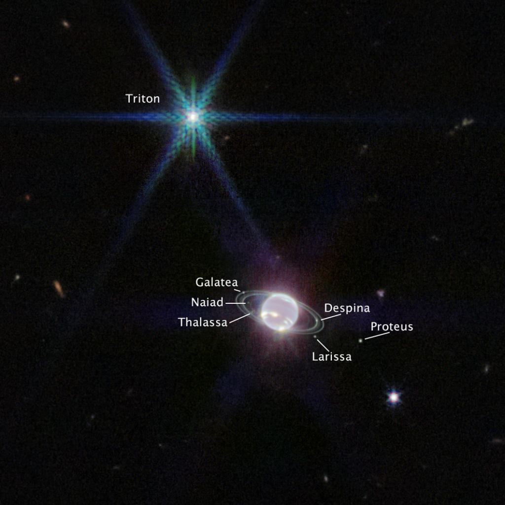
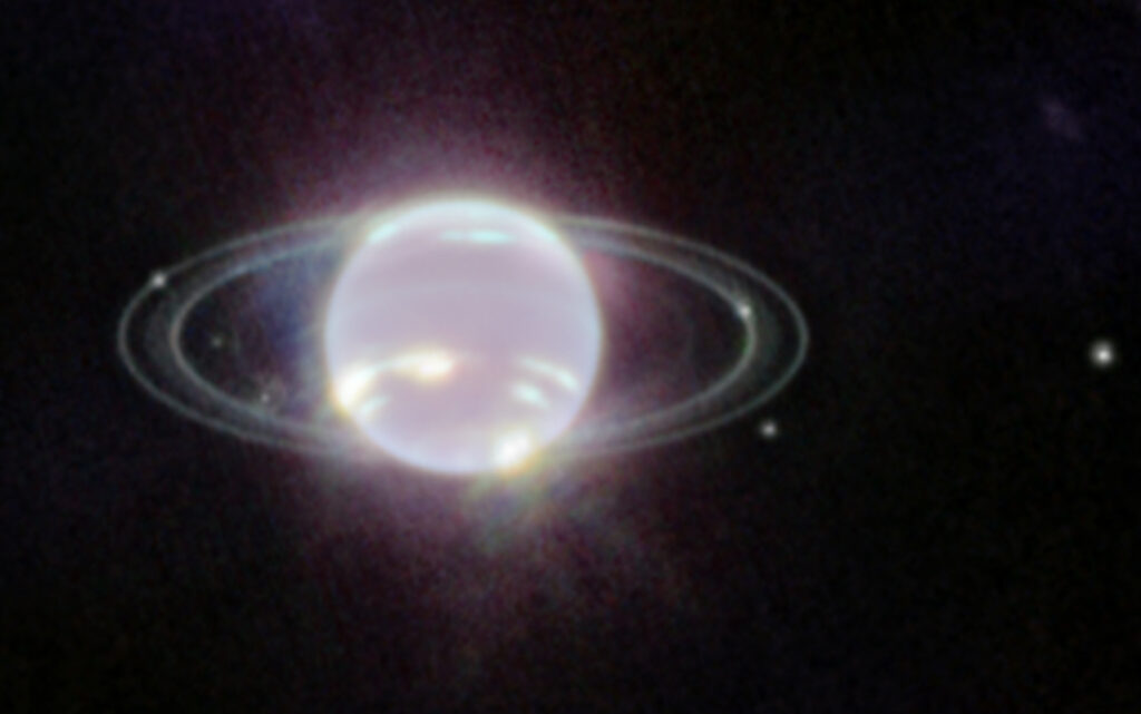
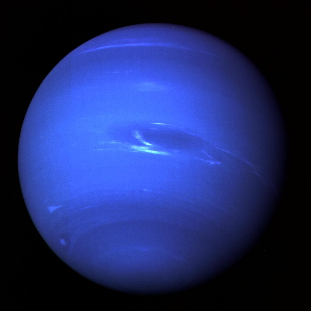
The Webb images of Neptune, taken on July 12, 2022, are reproduced below.
NASA: “Webb captured seven of Neptune’s 14 known moons: Galatea, Naiad, Thalassa, Despina, Proteus, Larissa, and Triton. Neptune’s large and unusual moon, Triton, dominates this Webb portrait of Neptune as a very bright point of light sporting the signature diffraction spikes seen in many of Webb’s images.” Source: NASA, ESA, CSA, STScINASA: “…image of Neptune……brings the planet’s rings into full focus for the first time in more than three decades. The most prominent features of Neptune’s atmosphere in this image are a series of bright patches in the planet’s southern hemisphere that represent high-altitude methane-ice clouds. More subtly, a thin line of brightness circling the planet’s equator could be a visual signature of global atmospheric circulation that powers Neptune’s winds and storms. Additionally, for the first time, Webb has teased out a continuous band of high-latitude clouds surrounding a previously-known vortex at Neptune’s southern pole.” Source: NASA, ESA, CSA, STScI
The Space Telescope Science Institute (STScI) has created a Resource Gallery of Webb Space Telescope images, which you can browse here: https://webbtelescope.org/resource-gallery/images. Currently there are 280 images in the Webb Resource Gallery. I think this is a website worth revisiting from time to time.
NASA’s Solar System Exploration website provides views of Neptune from several earlier sources, including the 1989 Voyager 2 deep space probe, the Hubble Space Telescope and the European Southern Observatory’s (ESO) Very Large Telescope (VLT). Check it out here: https://solarsystem.nasa.gov/planets/neptune/galleries/
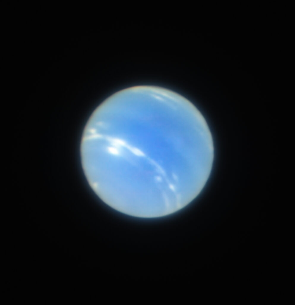
2018: The following image was taken in July 2018 during the testing of the narrow-field, adaptive optics mode of the optical/infrared MUSE/GALACSI instrument on ESO’s VLT, which is located at an elevation of 2,635 m (8,645 ft) at Cerro Paranal, in the Atacama Desert of northern Chile.
2018 VLT image of Neptune. The corrected image is sharper than a comparable image from the NASA/ESA Hubble Space Telescope. Source: ESO/P. Weilbacher (AIP)
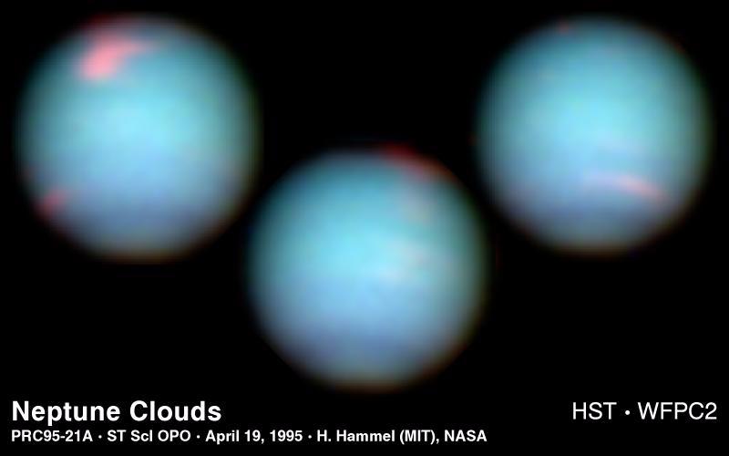
1994: The more recent Webb Space Telescope and VLT images are much better than the Hubble Space Telescope optical-range images of Neptune taken more than two decades earlier, in 1994.
NASA: “The images were taken in 1994 on October 10 (upper left), October 18 (upper right), and November 2 (lower center). Hubble is allowing astronomers to study Neptune’s dynamic atmosphere with a level of detail not possible since the 1989 flyby of the Voyager 2 space probe. Building on Voyager’s initial discoveries, Hubble is revealing that Neptune has a remarkably dynamic atmosphere that changes over just a few days. The temperature difference between Neptune’s strong internal heat source and its frigid cloud tops (-260 degrees Fahrenheit) might trigger instabilities in the atmosphere that drive these large-scale weather changes. In addition to hydrogen and helium, the main constituents, Neptune’s atmosphere is composed of methane and hydrocarbons, like ethane and acetylene.” Source: NASA, JPL, STScI
1989: In October 1989, the following whole planet view of Neptune was produced using images taken through the green and orange filters on the narrow angle camera during the Voyager 2 spacecraft flyby of the planet.
NASA: “This picture of Neptune was taken by Voyager 2 less than five days before the probe’s closest approach of the planet on Aug. 25, 1989. The picture shows the “Great Dark Spot” — a storm in Neptune’s atmosphere — and the bright, light-blue smudge of clouds that accompanies the storm”. Source: NASA/JPL-Caltech (1989)
In the future, we can hopefully look forward to more detailed multi-messenger images of Neptune, combining the near-infrared images from Webb with images from other observatories that can view the planet in different spectral bands.
The first-ever direct image of a black hole was released on 10 April 2019 by the Event Horizon Telescope (EHT) team and the National Science Foundation (NSF). The target for their observation was the supermassive M87* black hole at the center of the distant Messier 87 (M87) galaxy, some 54 million light years away. The EHT team estimated that M87* has a mass of about 6.5 billion Solar-masses (6.5 billion times greater than the mass of our Sun), and the black hole consumes the equivalent of about 900 Earth-masses per day. One Solar mass is roughly equivalent to the weight of the Sun and about 333,000 times the mass of Earth. Gases orbiting around the giant M87* black hole take days to weeks to complete an orbit. For more information on the first M87* black hole image, see my 10 April 2019 article here: https://lynceans.org/all-posts/the-event-horizon-telescope-team-has-produced-the-first-image-showing-the-shadow-of-a-black-hole/
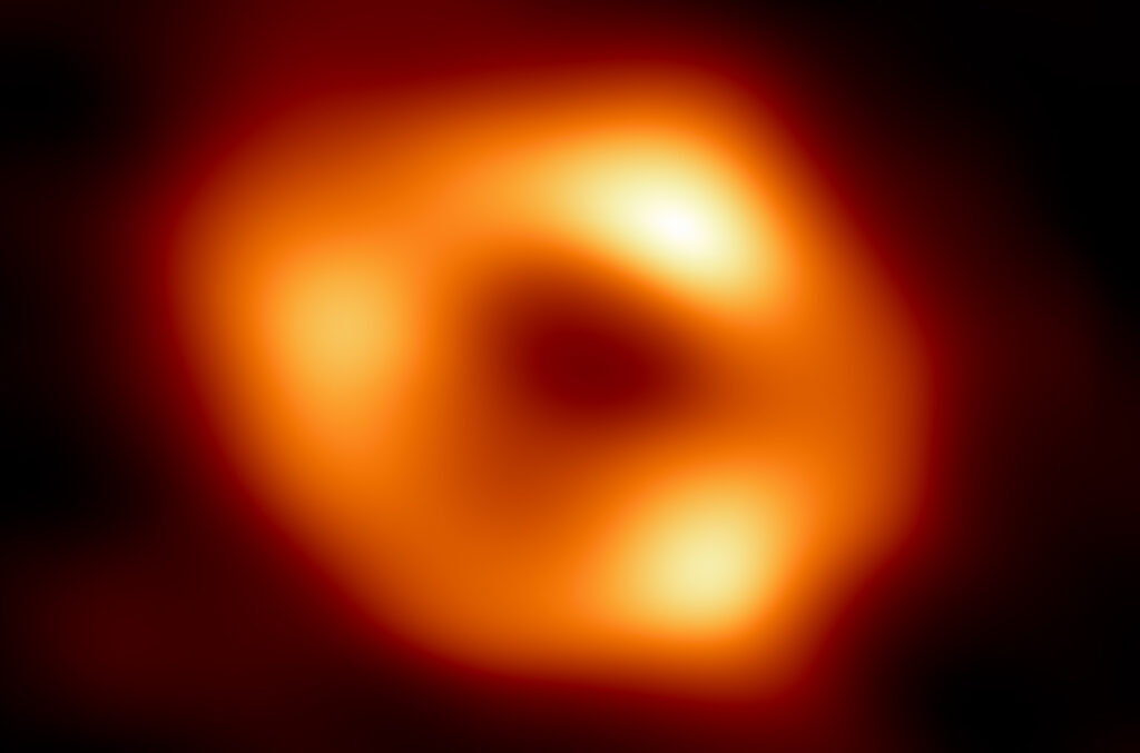
For decades, there has been mounting evidence that there is a massive black hole, known as Sagittarius A*, or Sgr A* for short, at the center of our Milky Way galaxy. Its presence has been inferred from the motions of visible stars that are orbiting under the gravitational influence of the black hole or are in the general vicinity of the black hole. Using observed data from more than 30 stars in the region around the galactic center, scientists developed high-resolution simulations that helped refine estimates of the location, mass and size of the Sgr A* black hole without having data from direct observations. For more information on this work, see my 24 January 2017 article here: https://lynceans.org/all-posts/the-black-hole-at-our-galactic-center-is-revealed-through-animations/
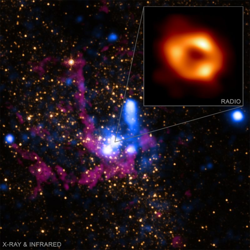
First-ever image looking down into the ring of rotating, glowing gas surrounding Sgr A*.Source: EHT CollaborationComposite image showing the location of the Sgr A* black hole (inset) in a composite X-ray/infrared NASA image of the heart of our Milky Way galaxy. Source: EHT Collaboration & NASA
Even though it was much closer than M87*, getting an image of Sgr A* was much harder because the Sgr A* black hole had to be viewed through the densely populated central plane of our Milky Way. The Sgr A* radio frequency (millimeter wave) observations were made in 2017 at a wavelength of 1.3 mm (230 GHz), the same as the first image of M87*.
Details that have emerged so far from the Sgr A* observation include the following.
Sgr A* is about 27,000 light years away, at the heart of our own galaxy (about 2 thousand times closer than M87*, which is in a different galaxy).
Sgr A* has a mass is about 4 million times the mass of our Sun, which is just a small fraction (1/1,500th , or 0.07%) of the mass of M87*.
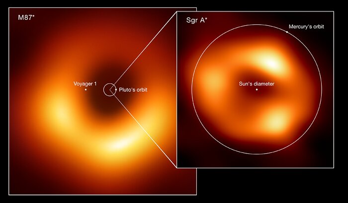
The glowing gas ring surrounding the Sgr A* black hole has an outer diameter of about 72 million miles (115 million km) across, which is approximately the diameter of Mercury’s orbit around the Sun in our solar system. The EHT team reported, “We were stunned by how well the size of the ring agreed with predictions from Einstein’s Theory of General Relativity.” By comparison, M87* is vastly larger, with the inner black hole region measuring about 23.6 billion miles (38 billion km) across (about 330 times the diameter of the entire Sgr A* black hole, including the glowing gas ring), as shown in the following scale diagram.
Comparison of the sizes of M87* (left) and Sgr A* (right). Source: EHT Collaboration (acknowledgment: Lia Medeiros)
The two black holes subtend approximately the same angle when viewed from Earth. The EHT team reported that the M87* bright emission disk subtends an angle of 42 ± 3 microarcseconds.
Gases orbiting around the Sgr A* black hole take mere minutes to an 1 hour to complete an orbit. The fast moving gases blur the image for an EHT observation typically lasting several hours. The released image of the Sgr A* black hole is an average of many different images the EHT team extracted from the data.
Sgr A* is far less active than M87*, and consumes only about 1/1,000th the mass per day (equivalent of about 1 Earth-mass per day).
The source of the three bright spots in the glowing gas ring are unknown at this time. They may be artifacts of the EHT observation process.
Follow-on EHT observations will benefit from additional telescopes joining the EHT network and significant technical improvements being made to the EHT telescopes and network systems. For example, operating the telescopes in the EHT array at a shorter wavelength of 0.87 mm (frequency of 345 GHz) will improve angular resolution by about 40%. More frequent observations and faster data processing would enable time-lapse movies to be created to show the dynamics of gas motion around the black hole. Details on planned improvements are discussed in my 9 April 2020 article here: https://lynceans.org/all-posts/working-toward-a-more-detailed-view-of-a-black-hole/
It is generally assumed that all of the observable objects in our universe in composed of ordinary matter. The rationale for this assumption if explained in a 1999 Scientific American article by Steve Naftilan: https://www.scientificamerican.com/article/how-do-we-know-that-dista/
In most of the electromagnetic spectrum, a star composed of normal matter and a star composed of antimatter (anti-star) will look the same to an observer on Earth. Their visible spectra will be indistinguishable. A key difference in behavior may be observable in the gamma ray spectrum, where high-energy gamma rays characteristic of matter-antimatter annihilation (i.e., baryon-antibaryon reactions) may reveal the identity of an antimatter star within our galaxy or an antimatter star cluster outside our galaxy. Luigi Foschini provides a good introduction to this subject in his 2000 paper at the following link: https://cds.cern.ch/record/447091/files/0007180.pdf
NASA’s Alpha Magnetic Spectrometer (AMS) has developed into an important tool in the search for anti-stars. The prototype, AMS-01 flew on the STS-91 Space Shuttle mission from 2 to 12 June 1998 and was successfully tested in orbit. The full-scale AMS-2 was launched aboard the STS-134 Space Shuttle mission on 16 May 2011. Since it was installed on the International Space Station (ISS) and activated on 19 May 2011, this 18,739 pound (8,500 kg), 2,250 cu. ft (64 cu meter) instrument has collected and analyzed more than 165 billion cosmic ray events (as of April 2021), and identified 9 million of these as antimatter, including the possible detection of antihelium nuclei.
You’ll find more information on AMS-1 and -2 on the NASA website here: https://ams.nasa.gov
AMS-2 installed on the ISS. Source: NASA
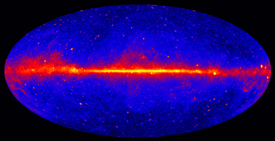
Another important source of data related to antimatter in our universe is NASA’s Fermi Gamma-ray Space Telescope, which was launched into a low Earth orbit on June 11, 2008. NASA’s website for the ongoing Fermi mission is here: https://fermi.gsfc.nasa.gov
The entire sky at gamma-ray energies greater than 1 GeV based on five years of data from Fermi’s Large Area Telescope (LAT) instrument. Brighter colors indicate brighter gamma-ray sources. Source: NASA/DOE/Fermi LAT Collaboration
In an 8 February 2021 article, astrophysicist Paul Sutter postulates the existence of antimatter star clusters that escaped the primordial matter-antimatter annihilations and now exist in relative isolation, for example, as an antimatter star cluster orbiting our Milky Way galaxy.
The antimatter stars in the cluster would continuously shed antimatter into the cosmos, leading to subsequent matter-antimatter interactions that produce high-energy particles that may be detectable from Earth.
Sutter commented, “…if astronomers are able to pinpoint a globular cluster as a particularly strong source of anti-particles, it would be like opening a time capsule, giving us a window into the physics that dominated the universe when it was only a second old.”
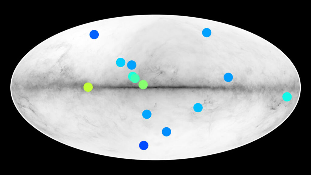
In a 20 April 2021 paper, authors Dupourqué, Tibaldo, and von Ballmoos report the possible detection of 14 anti-stars within our Milky Way galaxy. They used 10 years of data on 5,800 gamma-ray sources in Fermi’s data catalog to develop an estimate of the possible abundance of anti-stars. The authors report: “We identify in the catalog 14 anti-star candidates not associated with any objects belonging to established gamma-ray source classes and with a spectrum compatible with baryon-antibaryon annihilation.”
Fourteen celestial sources of gamma rays (colored dots in this all-sky map of the Milky Way; yellow / green indicates bright sources and blue shows dim sources) may come from stars made of antimatter. Source: Simon Dupourqué / IRAP via ScienceNews
The 14 anti-star candidates await further analysis to confirm or refute their existence. If confirmed, they represent only a small fraction of the population of all gamma-ray sources observed by the Fermi Gamma-ray Space Telescope. Nonetheless, even one confirmed anti-star would be a remarkable achievement.
For more information:
Steve Naftilan, “How do we know that distant galaxies are composed of matter rather than anti-matter? If equal quantities of each were produced in the big bang, might not some parts of the universe contain primarily matter and other parts primarily anti-matter?” Scientific American, 21 October 1999: https://www.scientificamerican.com/article/how-do-we-know-that-dista/
Simon Dupourqué, Luigi Tibaldo, and Peter von Ballmoos, “Constraints on the antistar fraction in the Solar System neighborhood from the 10-year Fermi Large Area Telescope gamma-ray source catalog,” Phys. Rev. D 103, 083016, 20 April 2021 (abstract only without subscription): https://journals.aps.org/prd/abstract/10.1103/PhysRevD.103.083016
Uranus, the seventh planet from the Sun, is an ice giant planet with 27 known moons in a unique orbit beyond Saturn. Uranus makes a complete orbit around the Sun in about 84 Earth years. It is the only planet whose equator is tilted nearly at a right angle to its orbital plane, which results in the polar regions pointing toward the Sun (and Earth) during parts of the orbit.
Uranus was visited briefly by NASA’s Voyager 2 spacecraft during its January 1986 flyby, which came within 81,500 km (50,600 miles) of the planet’s cloud tops. Since then, Uranus has been studied at visible, near-infrared and X-ray wavelengths from the perspective of terrestrial and near-Earth, space-based observatories.
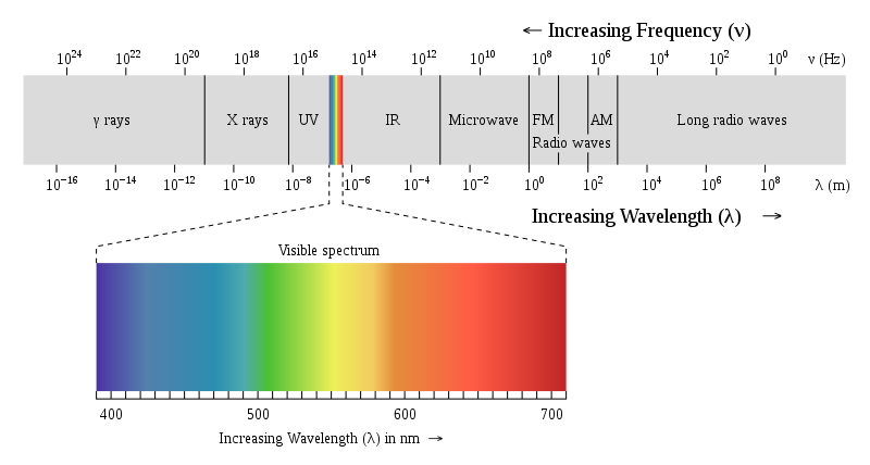
Visible light has a wavelength in the range from about 350 to 750 nanometers (nm, 10-9meters) or 3,500 to 7,500 Angstroms. Near-infrared light is the part of the infrared spectrum that is closest to the visible light spectrum, but at a longer wavelength, from about 800 to 2,500 nm. X-rays have a much shorter wavelength, from about 20 to 0.001 nm. In the following chart, you can see the relative placement of visible and near-infrared light and X-rays in the electromagnetic spectrum.
Electromagnetic spectrum. Source: Wikipedia
2. 2021 composite images of Uranus at visible / near-infrared and X-ray wavelengths
In March 2021, the National Aeronautics and Space Administration (NASA) announced that its orbiting Chandra X-ray Observatory had made the first ever detection of X-rays coming from the ice giant planet Uranus. Recent analysis of Chandra observations from 2002 and 2017 resulted in this discovery. You can read NASA’s 2021 announcement of this discovery here: https://chandra.si.edu/photo/2021/uranus/
X-rays coming from other planets have been detected in the past. NASA reported, “Like Jupiter and Saturn, Uranus and its rings appear to mainly produce X-rays by scattering solar X-rays, but some may also come from auroras…… The X-rays from auroras on Jupiter come from two sources: electrons traveling down magnetic field lines, as on Earth, and positively charged atoms and molecules raining down at Jupiter’s polar regions. However, scientists are less certain about what causes auroras on Uranus.”
Another possible X-ray source could be from an interaction between Uranus’ rings and the near-space charged particle environment around the planet. This phenomenon has been observed at Saturn.
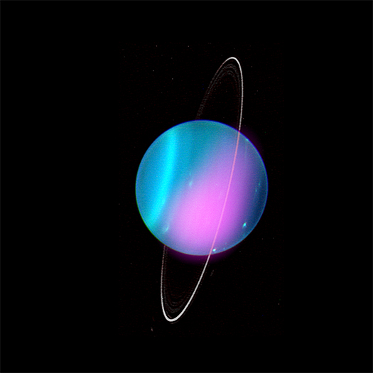
In connection with the discovery of X-rays coming from Uranus, NASA released two spectacular composite (multi-messenger) images of the planet created by combining images from two different parts of the electromagnetic spectrum: optical / near-infrared and X-ray.
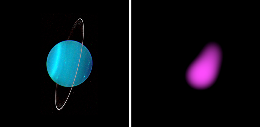
The components of the first composite image are described below:
Near-infrared image: This was taken in July 2004 with the 10-meter (32-foot 10-inch) Keck-1 telescope located at an altitude of 4,145 meters (13,599 ft) on Maunakea, Hawaii.
The X-ray image: This was produced with 7 August 2002 data from the Advanced CCD Imaging Spectrometer (ACIS) aboard Chandra, which has a spatial resolution of 0.5” (seconds). The angular size of Uranus for the observation was 3.7”. The X-rays were in the 0.6 to 1.1 keV (2.1 to 1.1 nm) spectral range, which is consistent with X-ray emissions from Jupiter and Saturn.
(Left) Keck-1 July 2004 near-infrared image of Uranus. The North Pole is at the 4 o’clock position. Sources: Space Science Institute; University of Wisconsin-Madison / W. M. Keck Observatory (Right) Chandra August 2002 ACIS X-ray image of Uranus. Sources: NASA/CXO/University College London
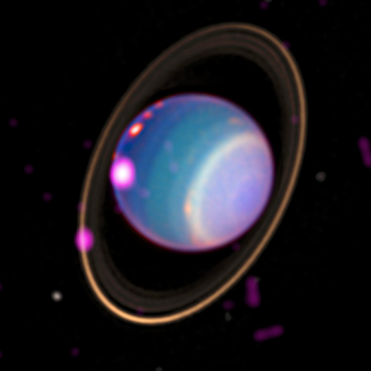
2021 Keck-1 & Chandra ACIS composite image
The second 2021 composite image, shown below, was created from a Keck optical image and X-ray images made with Chandra’s High Resolution Camera (HRC) during observations on 11 and 12 November 2017. The HRC is sensitive to softer X-ray emissions (down to 0.06 keV, 20.7 nm) than ACIS, enabling it to collect more photons in the 0.1–1.2 keV (12.4 to 0.1 nm) range most important for planetary studies. The authors report, ”These fluxes exceed expectations from scattered solar emission alone, suggesting either a larger X-ray albedo than Jupiter/Saturn or the possibility of additional X-ray production processes at Uranus.”
2021 Keck & Chandra HRC composite image Sources: X-ray: NASA/CXO/University College London/W. Dunn et al; Optical: W.M. Keck Observatory
The authors conclude by noting that, “Further, and longer, observations with Chandra would help to produce a map of X-ray emission across Uranus and to identify, with better signal-to-noise, the source locations for the X-rays, constraining possible contributions from the rings and aurora…… However, the current generation of X-ray observatories does not provide sufficient sensitivity to spectrally characterize the short interval temporal fluctuation observed in the November 12, 2017 observation.”
New space-based X-ray observational capabilities are being developed by NASA and the European Space Agency (ESA), but won’t be operational for a decade or more:
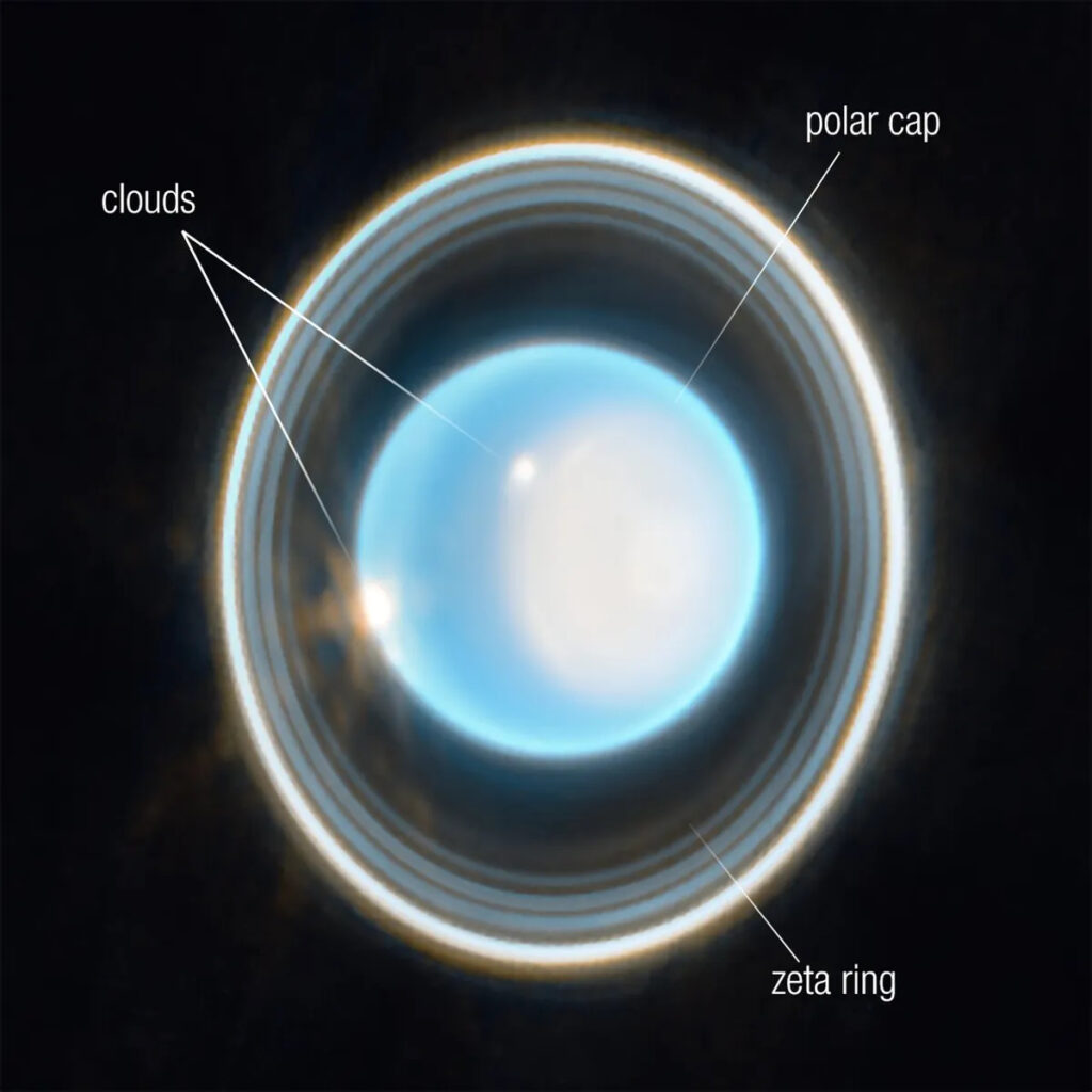
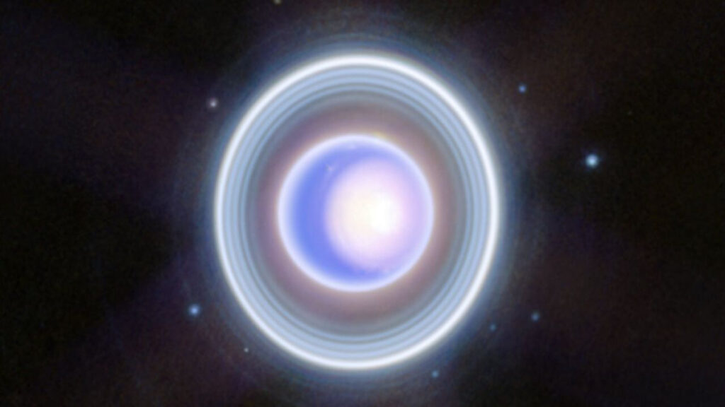
The James Webb Space Telescope (JWST), which has four science instruments designed to observe at optical to mid-infrared (0.6 – 28.3 microns) wavelengths, produced its first images of Uranus in April 2023.
Annotated image of Uranus captured by the JWST on 6 Feb. 2023, provides a view of the bright North polar ice cap and glowing clouds at near-infrared wavelengths of 1.4 to 3.0 microns.Sources: NASA, ESA, CSA, STScI
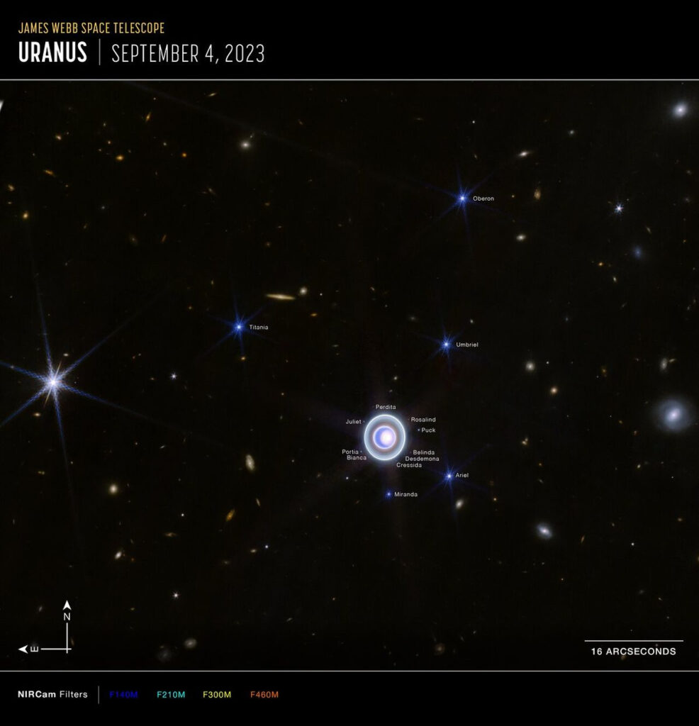
Wide field image of Uranus captured by the JWST on 6 Feb. 2023 at near-infrared wavelengths of 1.4 to 5.0 microns. Note that 14 of the 27 known moons are identified in the image. Also note the many distant galaxies in this image. Sources: NASA, ESA, CSA, STScI
Enlarged view of the 6 Feb. 2023 JWST near-infrared image shows the bright North polar cap, glowing clouds, details of the ring structure and many of the inner moons. Sources: NASA, ESA, CSA, STScI
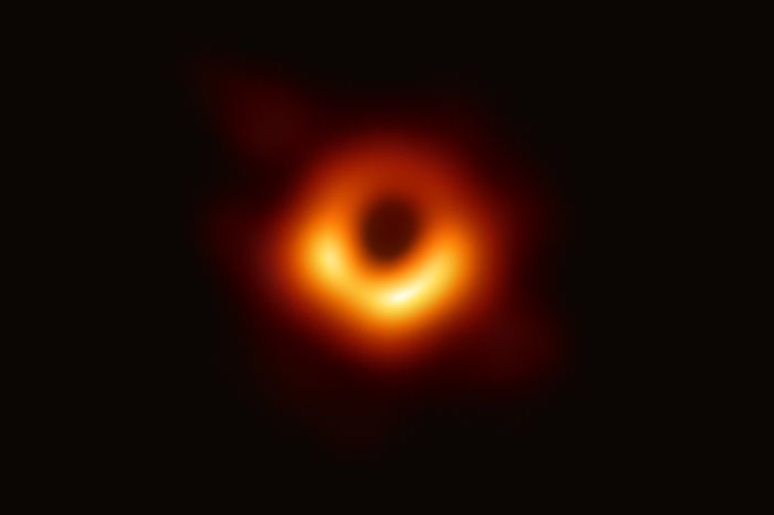
The first image of the shadow of a black hole was released on 10 April 2019 by the Event Horizon Telescope (EHT) collaboration and the National Science Foundation (NSF). The target of their observation was the supermassive black hole located near the center of the Messier 87 (M87) galaxy, which is about 55 million light years from Earth. That black hole is estimated to have a mass 6.5 billion times greater than our Sun.
Non-polarized image of M87 released 10 April 2019. Source: EHT & NSF
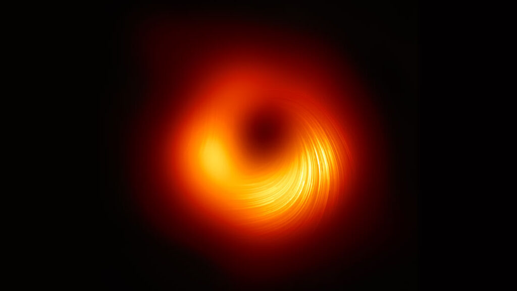
After further analysis of the historic M87 data, EHT astronomers have been able to measure the polarization of the radio frequency signals from the bright disk of the black hole. Polarization is a signature of the direction of the very strong magnetic fields in the hot glowing gas at the edge of a black hole, which can be seen in the following image released on 24 March 2021.
Polarized image of M87 released 24 March 2021. Source: EHT
The ability to measure the polarization in fine detail provides a new tool for mapping the dynamic magnetic field structure of a black hole. The new image shows the magnetic fields in the swirling accretion disk, which contains matter that is falling into the black hole.
Researchers also measured polarization that is pointing directly toward or away from the black hole, perpendicular to the accretion disk. Very strong magnetic fields in these directions may be responsible for launching plasma jets into space, away from the black hole. Such jets have been observed emanating from some black holes.
These are exciting times in astronomy and astrophysics.
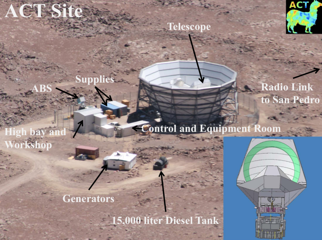
The Atacama Cosmology Telescope (ACT) is a six-meter (19.7 foot) radio telescope designed to make high-resolution, microwave-wavelength surveys of the cosmic microwave background (CMB). It is located at a remote site in the Atacama Desert at an elevation of 5,190 meters (17,030 feet) in northern Chile.
The ACT site. Source: ACT Collaboration
ACT observes in three frequency bands (148, 218 and 277 GHz) and has a resolution of 1.3 arc minutes at 148 GHz, near the peak of the CMB spectrum. This is significantly higher than the 5-10 arc minute resolution of the Planck spacecraft, which observed the CMB from 2009 to 2013 in the frequency range from 30 to 857 GHz. You’ll find a detailed description of the Atacama Cosmology Telescope (ACT) at the following link: https://www.cosmos.esa.int/documents/387566/387653/Ferrara_Dec3_09h20_Devlin_ACT.pdf
New results from the ACT survey, reported in December 2020, affirm the Planck CMB survey results.
The universe is isotropic
The estimate of the age of the universe was refined to 13.77 billion years old ± 0.04 billion years, overlapping uncertainty bands with the 2015 Planck estimate of 13.813 ± 0.038 billion years
The value of the Hubble constant was refined to 67.6 kilometers / second / megaparsec, up slightly from the 2018 Planck estimate of 67.4 kilometers / second / megaparsec. The significant difference from the value derived from astrophysical measurements, 73.5 km / second / megaparsec, remains unexplained.
ACT high resolution image of the isotropic cosmic background radiation covering a section of the sky 50 times the width of a full moon. This image represents a region of space 20 billion light-years across. Source: ACT Collaboration via EarthSky
For more information:
S.K. Choi, et al., “The Atacama Cosmology Telescope: a measurement of the Cosmic Microwave Background power spectra at 98 and 150 GHz,” Journal of Cosmology and Astroparticle Physics (subscription required), Volume 2020, December 2020: https://iopscience.iop.org/article/10.1088/1475-7516/2020/12/045/pdf
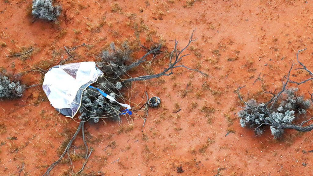
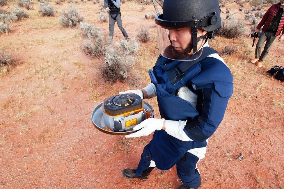
Japan’s Hayabusa2 (Japanese for Peregrine falcon 2) spacecraft returned from its six-year mission to asteroid 162173 Ryugu for a high-speed fly-by of Earth on 5 December 2020, during which it released a reentry capsule containing the material collected during two separate sampling visits to the asteroid’s surface. The capsule successfully reentered Earth’s atmosphere, landed in the planned target area in Australia’s Woomera Range and was recovered intact. The sample return capsule is known as the “tamatebako” (treasure box).
Location of Woomera Range. Source: itea.org
Hayabusa2’s sample return capsule after landing in the Woomera Range, Australia. Source: JAXACapsule containing samples from asteroid Ryugu. Source: JAXA
Background
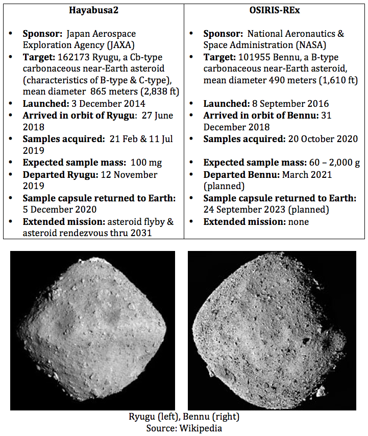
The first asteroid sample return mission was Japan’s Hayabusa1, which was launched on 9 May 2003 and rendezvoused with S-type asteroid 25143 Itokawa in mid-September 2005. A small sample was retrieved from the surface on 25 November 2005. The sample, comprised of tiny grains of asteroidal material, was returned to Earth on 13 June 2010, with a landing in the Woomera Range.
Japan’s Hayabusa2 and the US OSIRIS-Rex asteroid sample return missions overlap, with Hayabusa2 launching about two years earlier and returning its surface samples almost three years earlier. Both spacecraft were orbiting their respective asteroids from 31 December 2018 to 12 November 2019.
You’ll find a great deal of information and current news on the Hayabusa2 and OSIRIS-REx asteroid sample return missions on their respective project website:
An extended mission to explore additional asteroids was made possible by the excellent health of the Hayabusa2 spacecraft and the economic use of fuel during the basic mission. Hayabusa2 still has 30 kg (66 lb) of xenon propellant for its ion engines, about half of its initial load of 66 kg (146 lb).
As of September 2020, JAXA’s plans are is to target the Hayabusa2 spacecraft for the following two asteroid encounters:
Conduct a high-speed fly-by of L-type asteroid (98943) 2001 CC21 in July 2026. This asteroid has a diameter between 3.47 to 15.52 kilometers (2.2 to 9.6 miles).
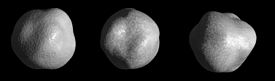
Continue on a rendezvous with asteroid 1998 KY26 in July 2031. This is a 30-meter (98-foot) diameter asteroid, potentially X-type (metallic), and rotating rapidly with a period of only 10.7 minutes.
Computer model view of 1998 KY26 based on radar data from Goldstone observatory. Source: NASA/JPL via Wikipedia
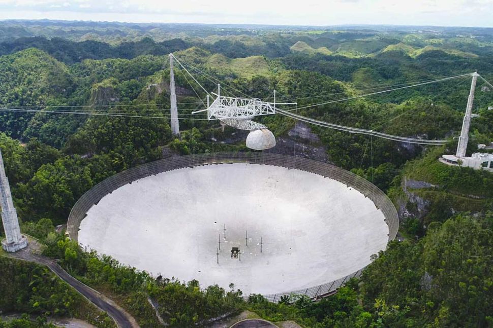
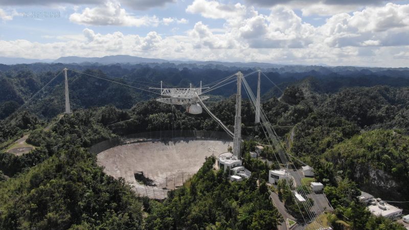
The Arecibo Observatory (AO) on Puerto Rico has been out of service since 10 August 2020, when a three-inch auxiliary support cable slipped out of its socket and fell onto the fragile radio telescope dish below. Three months later, on 6 November 2020, a second cable associated with the same support tower broke, damaging nearby cables, causing more damage to the reflector dish, and leaving the radio telescope’s support structure in a weakened and uncertain state.
On 19 November 2020, the National Science Foundation (NSF) announced it has begun planning for decommissioning the 57-year old Arecibo Observatory’s (AO) 1,000-foot (305-meter) radio telescope due to safety concerns after the two support wires broke and seriously damaged the antenna. You can read NSF News Release 20-010 at the following link: https://www.nsf.gov/news/news_summ.jsp?cntn_id=301674
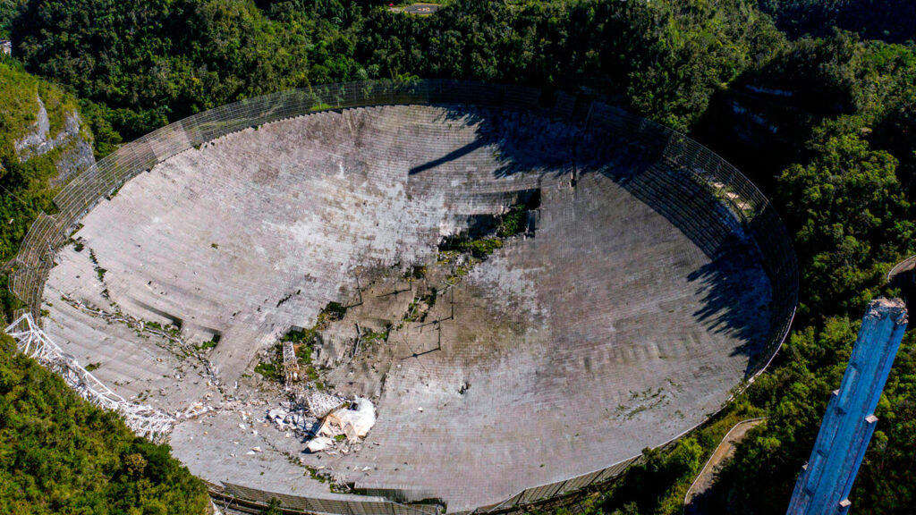
The 1,000-foot (305-m) dish at Arecibo Observatory in better days, in Spring 2019. Source: AO/University of Central Florida (UCF)The damaged Arecibo Observatory radio telescope in November 2020. Source: NSFA view from under the damaged dish. Source: AO/University of Central Florida (UCF)
Not included in the NSF timeline is the 1974 first-ever broadcast into deep space of a powerful signal that could alert other intelligent life to our technical civilization on Earth. The 1,679 bit “Arecibo Message” was directed toward the globular star cluster M13, which is 22,180 light years away. The message will be in transit for another 22,134 years.
A key capability lost is AO’s planetary radar capability that enabled the large dish to function as a high-resolution, active imaging radar. You’ll find examples of AO’s radar images of the Moon, planets, Jupiter’s satellites, Saturn’s rings, asteroids and comets on the NSF website here: https://www.naic.edu/~pradar/radarpage.html
More impressive than the still images were animations created from a sequence of AO radar images, particularly of passing asteroids. The animations defined the motion of the object as it flew near Earth. As an example, you can watch the following short (1:07 minutes) video, “Big asteroid 1998 OR2 seen in radar imagery ahead of fly-by”:
The US still has a reduced capability for planetary radar imaging with NASA’s Deep-Space Network’s Uplink Array.
The 19 November 2020 NSF news release stated, “After the telescope decommissioning, NSF would intend to restore operations at assets such as the Arecibo Observatory LIDAR facility — a valuable geospace research tool — as well as at the visitor center and offsite Culebra facility, which analyzes cloud cover and precipitation data.”
Adieu to radio astronomy at Arecibo.
Update 1 December 2020: Arecibo radio telescope collapsed.
NPR reported, “The Arecibo Observatory in Puerto Rico has collapsed, after weeks of concern from scientists over the fate of what was once the world’s largest single-dish radio telescope. Arecibo’s 900-ton equipment platform, suspended 500 feet above the dish, fell overnight after the last of its healthy support cables failed to keep it in place. No injuries were reported, according to the National Science Foundation, which oversees the renowned research facility.”
Arecibo after the collapse. Source: Ricardo Arduengo / AFP via Getty Images
Update 8 December 2020: National Science Foundation video shows the moment of collapse.
Update 19 October 2022: No NSF funding
On 18 October 2022, Science magazine reported on NSF’s plans to convert the iconic observatory in Puerto Rico into a center for education and outreach in science, technology, engineering, and math (STEM). The limited funding available for this purpose “does not include support for remaining instruments at the site, including a 12-meter radio telescope, a radio spectrometer, and a suite of optical laser instruments for studying the upper atmosphere.”
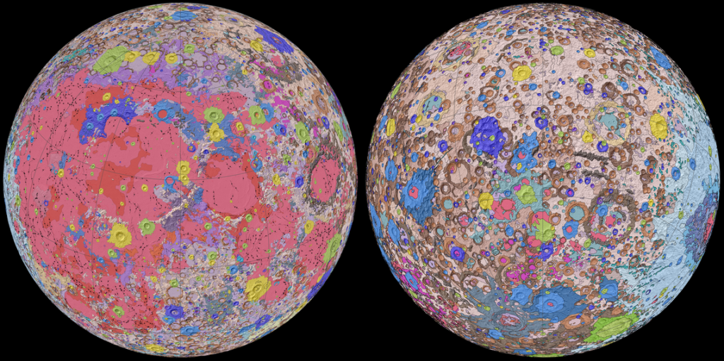
On 20 April 2020, the U.S. Geological Survey (USGS) released the first-ever comprehensive digital geologic map of the Moon. The USGS described this high-resolution map as follows:
“The lunar map, called the ‘Unified Geologic Map of the Moon,’ will serve as the definitive blueprint of the moon’s surface geology for future human missions and will be invaluable for the international scientific community, educators and the public-at-large.”
Color-coded orthographic projections of the “Unified Geologic Map of the Moon” showing the geology of the Moon’s near side (left) and far side (right). Source: NASA/GSFC/USGS
This remarkable mapping product is the culmination of a decades-long project that started with the synthesis of six Apollo-era (late 1960s – 1970s) regional geologic maps that had been individually digitized and released in 2013 but not integrated into a single, consistent lunar map.
This intermediate mapping product was updated based on data from the following more recent lunar satellite missions:
The Lunar Reconnaissance Orbiter Camera (LROC) is a system of three cameras that capture high resolution black and white images and moderate resolution multi-spectral images of the lunar surface: http://lroc.sese.asu.edu
Topography for the north and south poles was supplemented with Lunar Orbiter Laser Altimeter (LOLA) data: https://lola.gsfc.nasa.gov
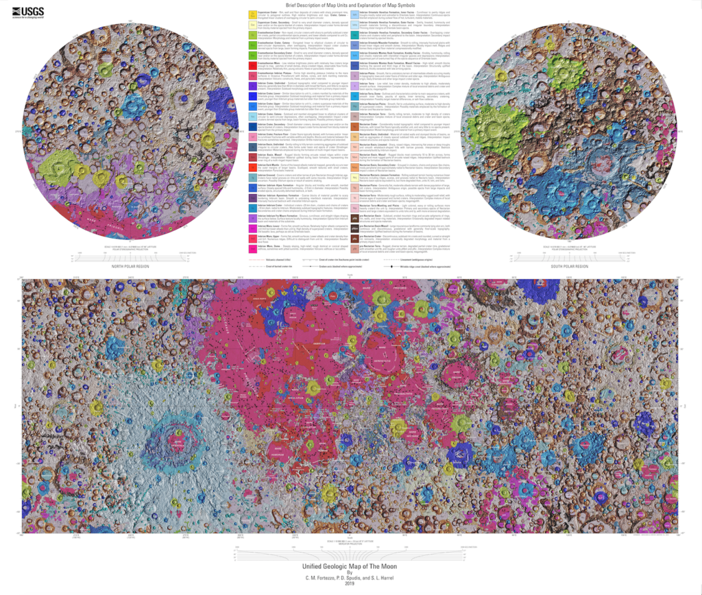
The final product is a seamless, globally consistent map that is available in several formats: geographic information system (GIS) format at 1:5,000,000-scale, PDF format at 1:10,000,000-scale, and jpeg format.
At the following link, you can download a large zip file (310 Mb) that contains a jpeg file (>24 Mb) with a Mercator projection of the lunar surface between 57°N and 57°S latitude, two polar stereographic projections of the polar regions from 55°N and 55°S latitudes to the poles, and a description of the symbols and color coding used in the maps.
These high-resolution maps are great for exploring the lunar surface in detail. A low-resolution copy (not suitable for browsing) is reproduced below.
For more information on the Unified Geologic Map of the Moon, refer to the paper by C. M. Fortezzo, et al., “Release of the digital Unified Global Geologic Map of the Moon at 1:5,000,000-scale,” which is available here: https://www.hou.usra.edu/meetings/lpsc2020/pdf/2760.pdf