This is a radioactivity-free vodka produced by The Chernobyl Spirit Company from grain and water in Chernobyl’s abandoned zone. The website for ATOMIK vodka is at the following link: https://www.atomikvodka.com
While this product has been widely reported in that past few days, the website offers the following notice:
“WARNING: Sorry, but we’ve only got one experimental bottle of ATOMIK so far, so we can’t sell you anything yet. But if you want to find out more about what we’re trying to do please carry on reading.”
The website is quite interesting and I encourage you to take the time to visit the site. Following is a summary of some key points from the website and a supporting technical paper.
Background
The members of the ATOMIK vodka technical team are:
Jim Smith, Professor of Environmental Science at Portsmouth University, UK
Gennady Laptev, Head of the Radiometric Laboratory at the Ukrainian Hydrometeorological Institute
Kyrylo Korychensky, a geologist and radiochemist currently completing his PhD at the Ukrainian Hydrometeorological Institute. Kyrylo’s family has long experience of distillation and he is the Master Distiller of ATOMIK grain spirit.
The team explained their basis for creating ATOMIK vodka.
“Our group of Ukrainian and UK scientists has been studying the transfer of radioactivity to crops both in the main Exclusion Zone (CEZ) and in the Narodychi District within the Zone of Obligatory Resettlement, where land can’t officially be used for agriculture, but people still live.
The research shows that in many areas land could now be used to produce crops, which are safe to eat. As every chemist knows, distillation of fermented grain leaves many heavier elements in the waste product so the distillate alcohol is more radioactively “pure” than the original grain. We have used distillation to reduce radioactivity in the grain even further to make a product from Chernobyl which we hope people will want to consume.”
The ATOMIK vodka product
The ATOMIK website contains the following description of the product.
“ATOMIK is a grain spirit (or “moonshine”), a homemade vodka made by people in villages all over Ukraine, Belarus, Poland and Russia since about the twelfth century.
Grain spirit has more flavour compounds than vodka – by double-distilling and filtering, we are trying to produce a grain spirit which keeps the flavour and character of homemade vodka (“samogon”) but isn’t quite as rough around the edges. We dilute our distillate with a mineral water from the deep aquifer below the town of Chernobyl about 10 km south of the nuclear power station. It is pure and of high quality, having characteristics of a typical limestone aquifer such as that found in the South of England or the Champagne region of France. We’re currently trying to work out exactly how many thousands of years old this water is but it definitely wasn’t anywhere near the surface in 1986.”
The distillate alcohol experiment
On the Atomic vodka website, the technical team reported on their radiochemical analysis of ATOMIK:
“We have been doing studies to see how much radioactivity transfers from soil to crops in the Chernobyl abandoned areas more than 30 years after the accident. We found that, at our site in the main exclusion zone, radiocaesium in rye was below the (quite cautious) Ukrainian limit but that radiostrontium was a bit above the limit. But when we made ATOMIK grain spirit from the grain, we could find no Chernobyl-derived radioactivity in the distilled alcohol.
The water used to dilute the distillate to 40% alcohol is a mineral water from the deep aquifer below the town of Chernobyl about 10 km south of the nuclear power station
The laboratories of The Ukrainian Hydrometeorological Institute and the University of Southampton GAU-Radioanalytical could find no trace of Chernobyl radioactivity in ATOMIK grain spirit. Out of scientific curiosity we’re going to try even more sensitive analytical methods to see if we can find something – nothing on Earth is completely free of radioactivity.”
The August 2019 technical report, “Distillate ethanol production for re-use of abandoned lands – an analysis and risk assessment,” by Jim Smith, Gennady Laptev, et al., shows the location of the experimental plot for ATOMIK grain harvesting relative to the areas around the Chernobyl site that were contaminated by Cs-137. The site is in an area that received a relatively low level of Cs-137 contamination.
Source: J. Smith, G. Laptev, et al., 2019
This report summarizes the results of the analysis as follows:
The rye grain had elevated levels of Cs-137 and Sr-90, but Pu and Am isotopes were below detection limits. The Sr-90 activity was slightly above the Ukrainian limit of 20 Bq kg-1.
There were no artificial radionuclides observed in the distillate ethanol (diluted to 40% with Chernobyl Town groundwater) sample.
The low energy beta analysis recorded an estimated 58 Bq/L, which we attribute to natural C-14 consistent with the expected activity concentration of natural C-14 in ethanol at this dilution.
It seems that ATOMIK is as safe to drink as any comparable grain spirit.
When The Chernobyl Spirit Companyis able to offer ATOMIK for sale, a key market will be the increasing number of tourists who now visit the Chernobyl exclusion zone. The Chernobyl Spirit Companyhas stated that at least 75% of profits from sales of ATOMIK will go to supporting communities in the affected areas and wildlife conservation.
While you can use the toast ‘na zdorovya’ in Ukraine, a more traditional Ukrainian toast is ‘budmo’ (cheers). When you hear the toast ‘budmo,’ reply back with a hearty ‘hey’! Keep that toast and reply cycle going and the evening will go by very quickly.
Best wishes for success to the The Chernobyl Spirit Company. I’m looking forward the day when I can get a bottle of ATOMIK at my local liquor store.
In my 21 May 2018 post, I reported on the pregnancy of the San Diego Zoo’s southern white rhino Victoria. The pregnancy was the result of artificial insemination on 22 March 2018 using the semen from another southern white rhino. This was the first time that San Diego Zoo Global’s Rhino Rescue Center had been successful in initiating a southern white rhino pregnancy through artificial insemination.
The healthy baby was born on 28 July 2019 after a gestation period of 493 days.
Victoria and baby. Source: San Diego Zoo Global
You can watch a short video of Victoria, the new baby, and San Diego Zoo Global’s Dr. Barbara Durrant here:
You may recall Dr. Barbara Durrant’s 21 June 2017 presentation to the Lyncean Group (Meeting # 112), “Endangered Species Rescue: How far should we go?” In this presentation, Dr. Durrant explained the complex process being developed at San Diego Zoo Global to use northern white rhino tissue to create artificial embryonic stem cells that can be matured into northern white rhino egg and sperm cells. You can see her 2017 presentation here:
There are only two northern white rhinos still alive in the whole world. Both are female and beyond breeding age. San Diego Zoo Global’s Rhino Rescue Centeris part of a team that is working to develop artificial insemination and embryo implantation techniques so they can reliably inseminate a northern white embryo into a southern white rhino female. This first successful birth of a southern white rhino as a result of artificial insemination is a key milestone in the process of saving the northern white rhino from extinction.
Congratulations to the team at San Diego Zoo Global’s Rhino Rescue Center and to Victoria for this important and happy milestone.
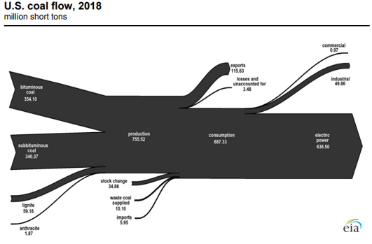
US coal production was strong from the 1990s until 2014, with coal production each year being near or above 1 billion short tons (a “short ton” is 2,000 pounds). The highest annual level of production was achieved in 2008: 1.17 billion short tons. Since then, the coal industry has seen a steady decline in production, and trends indicate that the decline will continue.
In their 10 July 2019 report, “Almost all US coal production is consumed by electric power,” the US Energy Information Administration (EIA) reported that coal is still one of the main sources of energy in the US, accounting for 16% of the nation’s primary energy production in 2018. Nearly all of the coal consumed in the US is produced domestically, and most is consumed by the electric power sector to generate electricity, while some is exported. The following EIA “coal flow” diagram shows where the coal comes from and (approximately) how it was consumed in 2018. Total production was about 755 million short tons. The electric power sector consumed about 84% of production, with only modest amounts being consumed by the industrial sector or exported.
Electricity generation from coal has been on the decline in the US for almost two decades. On 26 June 2019, EIA reported that US electricity generation from renewables surpasses coal in April 2019. In the following EIA chart, you can see the long-term increase in generation from renewables, which contrasts sharply with the long-term decline of generation from coal due to the decommissioning of many coal-fired power plan and the commissioning of no plants since about 2014.
Between 2010 and the first quarter of 2019, US power companies announced the retirement of more than 546 coal-fired power units, totaling about 102 gigawatts (GW) of generating capacity. Plant owners intend to retire another 17 GW of coal-fired capacity by 2025. You’ll find the EIA’s 26 July 2019 report on decommissioning US coal-fired power plants here: https://www.eia.gov/todayinenergy/detail.php?id=40212
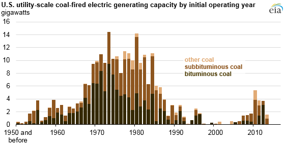
In April 2017, EIA reported that on the age of the US coal-fired generating plant fleet. The following chart shows the distribution of coal-fired plants based on their initial operating year. EIA reported a fleet average age of 39 years in 2017.
The following table lists EIA data on the numbers of different types of generating plants in the US between 2007 and 2017. In 2007, the US had 606 coal-fired generating plants. By the end of 2017, that number had dropped to 359.
In another decade, coal-fired generation will be only a small part of the US electric power generation portfolio and the average fleet age will be about 50 years old.
The National Oceanic and Atmospheric Administration’s (NOAA’s) National Centers for Environmental Information (NCEI) are responsible for “preserving, monitoring, assessing, and providing public access to the Nation’s treasure of climate and historical weather data and information.” The main NOAA / NCEI website is here:
The “State of the Climate” is a collection of monthly summaries recapping climate-related occurrences on both a global and national scale. Your starting point for accessing this collection is here:
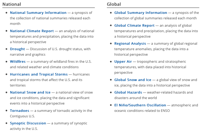
I’d like to direct your attention to two particularly impressive monthly summaries:
Global Summary Information, which provides a comprehensive top-level view, including the Sea Ice Index
Global Climate Report, which provides more information on temperature and precipitation, but excludes the Sea Ice Index information
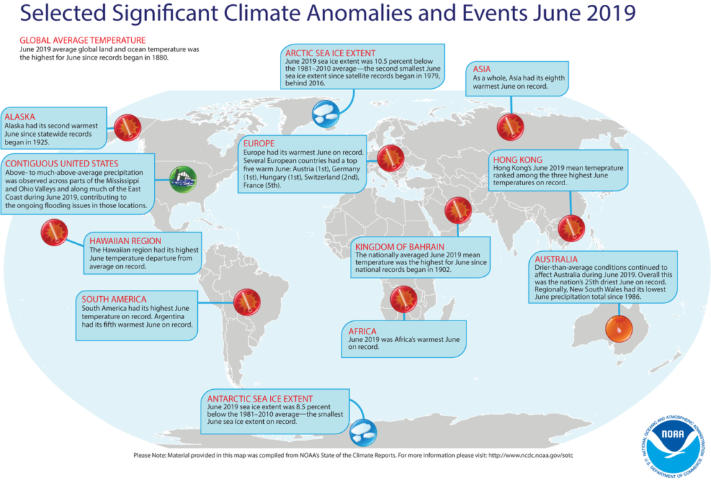
Here are some of the graphics from the Global Climate Report for June 2019.
Source: NOAA NCEISource: NOAA NCEI
NOAA offered the following synopsis of the global climate for June 2019.
The month of June was characterized by warmer-than-average temperatures across much of the world. The most notable warm June 2019 temperature departures from average were observed across central and eastern Europe, northern Russia, northeastern Canada, and southern parts of South America.
Averaged as a whole, the June 2019 global land and ocean temperature departure from average was the highest for June since global records began in 1880.
Nine of the 10 warmest Junes have occurred since 2010.
For more details, see the online June 2019 Global Climate Reportat the following link:
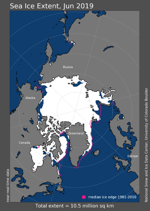
A complementary NOAA climate data resource is the National Snow & Ice Data Center’s (NSIDC’s) Sea Ice Index, which provides monthly and daily quick looks at Arctic-wide and Antarctic-wide changes in sea ice. It is a source for consistently processed ice extent and concentration images and data values since 1979. Maps show sea ice extent with an outline of the 30-year (1981-2010) median extent for the corresponding month or day. Other maps show sea ice concentration and anomalies and trends in concentration. In addition, there are several tools you can use on this website to animate a series of monthly images or to compare anomalies or trends. You’ll find the Sea Ice Index here:
The Arctic sea ice extent for June 2019 and the latest daily results for 23 July 2019 are shown in the following graphics, which show the rapid shrinkage of the ice pack during the Arctic summer. NOAA reported that the June 2019 Arctic sea ice extent was 10.5% below the 30-year (1981 – 2010) average. This is the second smallest June Arctic sea ice extent since satellite records began in 1979.
Source: NOAA NSIDC
Source: NOAA NSIDC
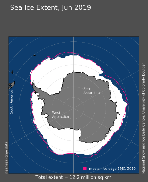
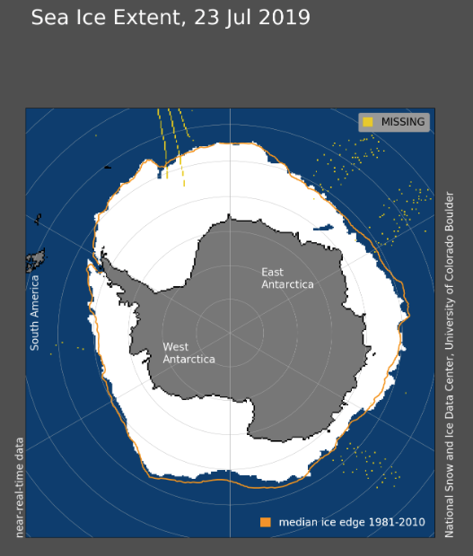
The monthly Antarctic results for June 2019 and the latest daily results for 23 July 2019 are shown in the following graphics, which show the growth of the Antarctic ice pack during the southern winter season. NOAA reported that the June 2019 Antarctic sea ice extent was 8.5% below the 30-year (1981 – 2010) average. This is the smallest June Antarctic sea ice extent on record.
Source: NOAA NSIDC
Source: NOAA NSIDC
I hope you enjoy exploring NOAA’s “State of the Climate” collection of monthly summaries.
On July 16th, 1969, 13:32:00 UTC, the Saturn V launch vehicle, SA-506, lifted off from Launch Pad 39-A at Kennedy Space Center, Florida on the Apollo 11 mission with astronauts Neil Armstrong (Mission commander), Michael Collins (Command Module pilot) and Edwin (Buzz) Aldrin (Lunar Module pilot).
L to R: Neil Armstrong, Michael Collins & Buzz Aldrin. Source: NASA
Apollo 11 insignia: Eagle with wings outstretched holding an olive branch above the Moon with Earth in the background.Source: NASA via Wikipedia
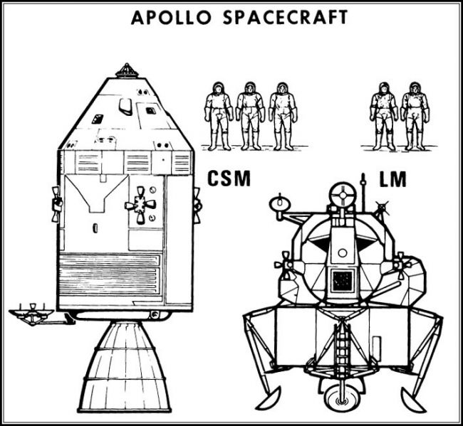
The Apollo spacecraft consisted of three modules:
The three-person Command Module (CM), named Columbia, was the living quarters for the three-person crew during most of the lunar landing mission.
The Service Module (SM) contained the propulsion system, electrical fuel cells, consumables storage tanks (oxygen, hydrogen) and various service / support systems.
The two-person, two-stage Lunar Module (LM), named Eagle, would make the Moon landing with two astronauts and return them to the CM.
The LM’s descent stage (bottom part of the LM with the landing legs) remained on the lunar surface and served as the launch pad for the ascent stage (upper part of the LM with the crew compartment). Only the 4.9 ton CM was designed to withstand Earth reentry conditions and return the astronauts safely to Earth.
General configuration of the Apollo spacecraft. The “CSM” is the combined Command Module and Service Module. Source: NASA
From its initial low Earth parking orbit, Apollo 11 flew a direct trans-lunar trajectory to the Moon, inserting into lunar orbit about 76 hours after liftoff. The Apollo 11 mission profile to and from the Moon is shown in the following diagram, and is described in detail here: https://www.mpoweruk.com/Apollo_Moon_Shot.htm
Source: NASA
Neil Armstrong and Buzz Aldrin landed the Eagle LM in the Sea of Tranquility on 20 July 1969, at 20:17 UTC (about 103 hours elapsed time since launch), while Michael Collins remained in a near-circular lunar orbit aboard the CSM. Neil Armstrong characterized the lunar surface at the Tranquility Base landing site with the observation, “it has a stark beauty all its own.”
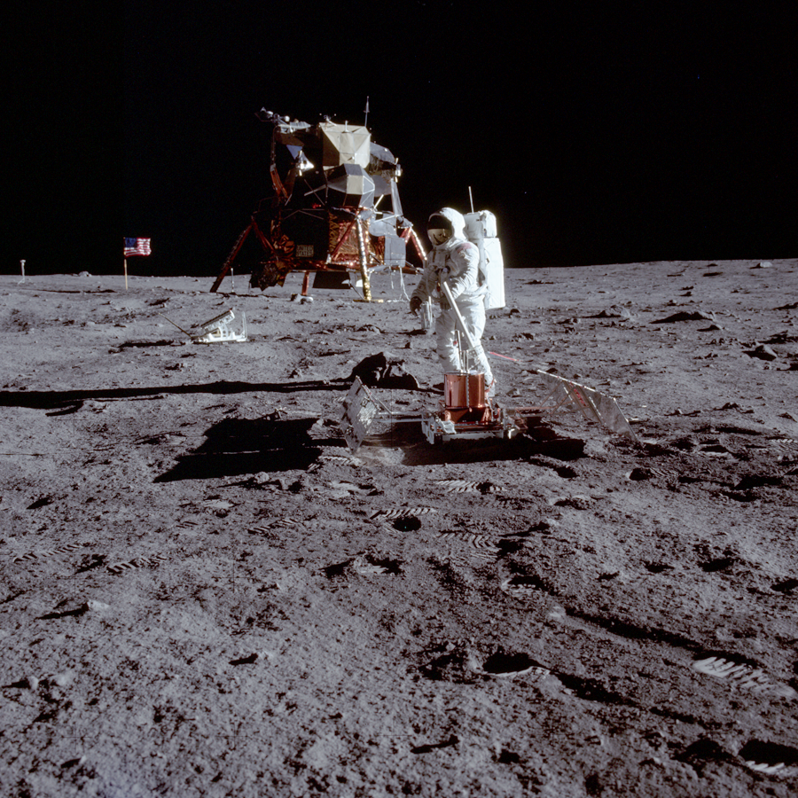
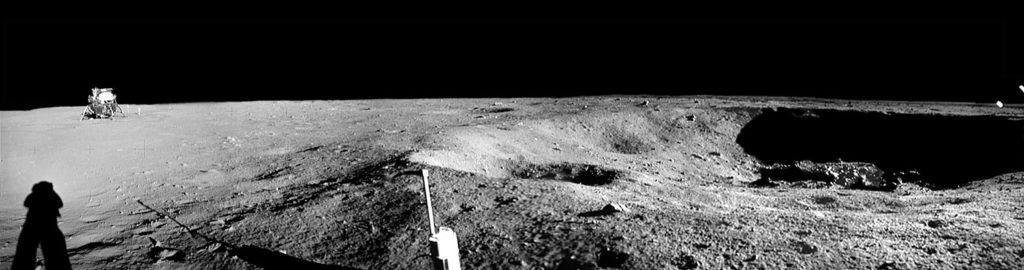
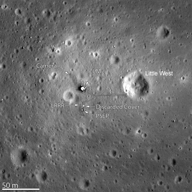
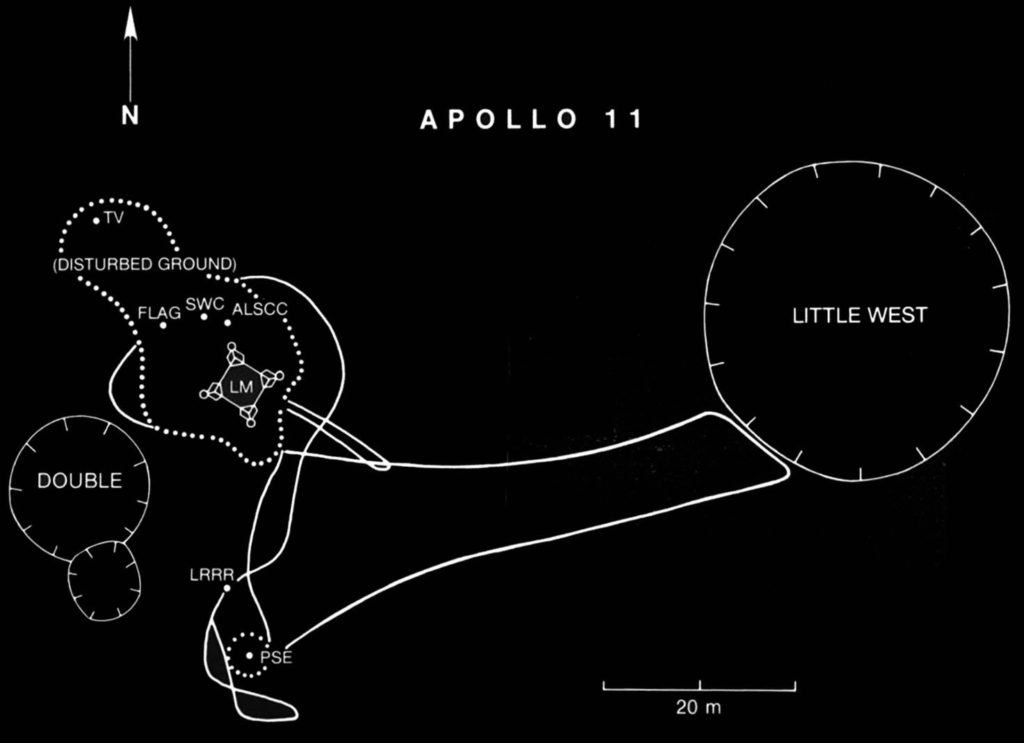
In the two and a half hours they spent on the lunar surface, Armstrong and Aldrin collected 21.55 kg (47.51 lb) of rock samples, took photographs and set up the Passive Seismic Experiment Package (PSEP) and the Laser Ranging RetroReflector (LRRR), which would be left behind on the Moon. The PSEP provided the first lunar seismic data, returning data for three weeks after the astronauts left, and the LRRR allows precise distance measurements to be collected to this day. Neil Armstrong made an unscheduled jaunt to Little West crater, about 50 m (164 feet) east of the LM, and provided the first view into a lunar crater.
Apollo 11 PSEP in the foreground with astronaut Buzz Aldrin and the LRRR behind it, then the Eagle LM, the American flag, and the TV camera on the left horizon beyond the American flag. Source: NASANeil Armstrong’s photo showing the Eagle LM from Little West crater (33 meters in diameter). Source: NASAApollo 11 landing site captured from 24 km (15 miles) above the surface by NASA’s Lunar Reconnaissance Orbiter (LRO). Source: adapted from NASA Goddard/Arizona State UniversityApollo 11 “traverse” map. Source: NASA via Smithsonian https://airandspace.si.edu/
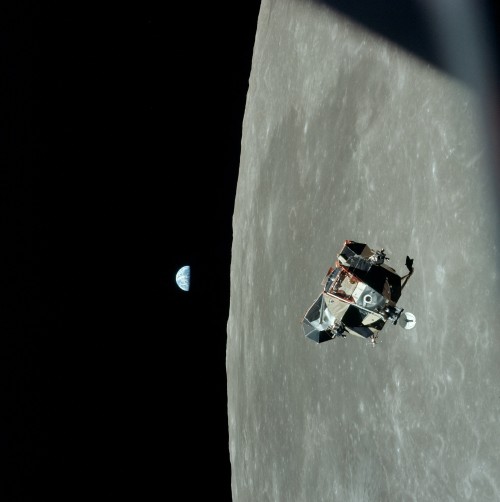
Armstrong and Aldrin departed the Moon on 21 July 1969 at 17:54 UTC in the ascent stage of the Eagle LM and then rendezvoused and docked with Collins in the CSM about 3-1/2 hours later.
LM Eagle ascent stage with Armstrong and Aldrin approaching the CSM Columbia piloted by Collins. Source: NASA
After discarding the ascent stage, the CSM main engine was fired and Apollo 11 left lunar orbit on 22 July 1969 at 04:55:42 UTC and began its trans-Earth trajectory. As the Apollo spacecraft approached Earth, the SM was jettisoned.
The CM reentered the Earth’s atmosphere and landed in the North Pacific on 24 July 1969 at 16:50:35 UTC. The astronauts and the Apollo 11 spacecraft were recovered by the aircraft carrier USS Hornet. President Nixon personally visited and congratulated the astronauts while they were still in quarantine aboard the USS Hornet. You can watch a video of this meeting here:
Mankind’s first lunar landing mission was a great success.
Postscript to the first Moon landing
A month after returning to Earth, the Apollo 11 astronauts were given a ticker tape parade in New York City, then termed as the largest such parade in the city’s history.
New York City ticker tape parade for the Apollo 11 astronauts. Source: NASA / Bill Taub
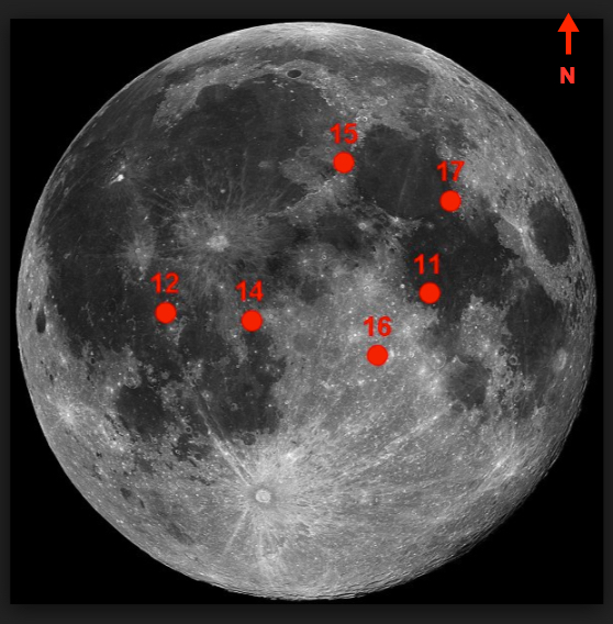
There were a total of six Apollo lunar landings (Apollo 11, 12, 14, 15, 16, and 17), with the last mission, Apollo 17, returning to Earth on 19 December 1972. Their landing sites are shown in the following graphic.
The Apollo landing sites. Source: NASA
In the past 46+ years since Apollo 17, there have been no manned missions to the Moon by the U.S. or any other nation.
Along with astronaut John Glenn, the first American to fly in Earth orbit, the three Apollo 11 astronauts were awarded the New Frontier Congressional Gold Medal in the Capitol Rotunda on 16 November 2011. This is the Congress’ highest civilian award and expression of national appreciation for distinguished achievements and contributions.
Neil Armstrong died on 25 August 2012 at the age of 82.
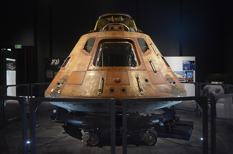
The Apollo 11 command module Columbia was physically transferred to the Smithsonian Institution in 1971 and has been on display for decades at the National Air and Space Museum on the mall in Washington D.C. For the 50th anniversary of the Apollo 11 mission, Columbia will be on display at The Museum of Flight in Seattle, as the star of the Smithsonian Institution’s traveling exhibition, “Destination Moon: The Apollo 11 Mission.” You can get a look at this exhibit at the following link: http://www.collectspace.com/news/news-041319a-destination-moon-seattle-apollo.html
The Apollo 11 command module Columbia at The Museum of Flight in Seattle. Source: collectSPACE
After years of changing priorities under the Bush and Obama administrations, NASA’s current vision for the next U.S. manned lunar landing mission is named Artemis, after the Greek goddess of hunting and twin sister of Apollo. NASA currently is developing the following spaceflight systems for the Artemis mission:
The Space Launch System (SLS) heavy launch vehicle.
A manned “Gateway” station that will be placed in lunar orbit, where it will serve as a transportation node for lunar landing vehicles and manned spacecraft for deep space missions.
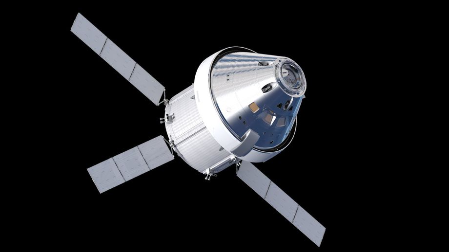
The Orion multi-purpose manned spacecraft, which will deliver astronauts from Earth to the Gateway, and also can be configured for deep space missions.
Lunar landing vehicles, which will shuttle between the Gateway and destinations on the lunar surface.
The Orion spacecraft is functionally comparable to the Apollo command and service modules. Source: NASA
While NASA has a tentative goal of returning humans to the Moon by 2024, the development schedules for the necessary Artemis systems may not be able to meet this ambitious schedule. The landing site for the Artemis mission will be in the Moon’s south polar region. NASA administrator Jim Bridenstine has stated that Artemis will deliver the first woman to the Moon.
Robert C. Seamens, Jr., “Project Apollo – The Tough Decisions,” NASA Monographs in Aerospace History Number 37, NASA SP-2007-4537, 2007; https://history.nasa.gov/monograph37.pdf
Ian A. Crawford, “The Scientific Legacy of Apollo,” Astronomy and Geophysics (Vol. 53, pp. 6.24-6.28), December 2012; https://arxiv.org/pdf/1211.6768.pdf
Roger D. Launis, “Apollo’s Legacy: Perspectives on the Moon Landings,” Smithsonian Books, 14 May 2019, ISBN-13: 978-1588346490
Neil Armstrong, Michael Collins & Edwin Aldrin, “First on the Moon,” William Konecky Assoc., 15 October 2002, ISBN-13: 978-1568523989
Michael Collins, “Flying to the Moon: An Astronaut’s Story,” Farrar, Straus and Giroux (BYR); 3 edition, 28 May 2019, ISBN-13: 978-0374312022
Michael Collins, “Carrying the Fire: An Astronaut’s Journeys: 50th Anniversary Edition Anniversary Edition,” Farrar, Straus and Giroux, 16 April 2019, ISBN-13: 978-0374537760
Edwin Aldrin, “Return to Earth,” Random House; 1st edition, 1973, ISBN-13: 978-0394488325
After the failure of Israel’s Beresheet spacecraft to execute a soft landing on the Moon in April 2019, India is the next new contender for lunar soft landing honors with their Chandrayaan-2 spacecraft. We’ll take a look at the Chandrayaan-2 mission in this post.
1. Background: India’s Chandrayaan-1 mission to the Moon
India’s first mission to the Moon, Chandrayaan-1, was a mapping mission designed to operate in a circular (selenocentric) polar orbit at an altitude of 100 km (62 mi). The Chandrayaan-1 spacecraft, which had an initial mass of 1,380 kg (3,040 lb), consisted of two modules, an orbiter and a Moon Impact Probe (MIP). Chandrayaan-1 carried 11 scientific instruments for chemical, mineralogical and photo-geologic mapping of the Moon. The spacecraft was built in India by the Indian Space Research Organization (ISRO), and included instruments from the USA, UK, Germany, Sweden and Bulgaria.
Chandrayaan-1 was launched on 22 October 2008 from the Satish Dhawan Space Center (SDSC) in Sriharikota on an “extended” version of the indigenous Polar Satellite Launch Vehicle designated PSLV-XL. Initially, the spacecraft was placed into a highly elliptical geostationary transfer orbit (GTO), and was sent to the Moon in a series of orbit-increasing maneuvers around the Earth over a period of 21 days. A lunar transfer maneuver enabled the Chandrayaan-1 spacecraft to be captured by lunar gravity and then maneuvered to the intended lunar mapping orbit. This is similar to the five-week orbital transfer process used by Israel’s Bersheet lunar spacecraft to move from an initial GTO to a lunar circular orbit.
The goal of MIP was to make detailed measurements during descent using three instruments: a radar altimeter, a visible imaging camera, and a mass spectrometer known as Chandra’s Altitudinal Composition Explorer (CHACE), which directly sampled the Moon’s tenuous gaseous atmosphere throughout the descent. On 14 November 2008, the 34 kg (75 lb) MIP separated from the orbiter and descended for 25 minutes while transmitting data back to the orbiter. MIP’s mission ended with the expected hard landing in the South Pole region near Shackelton crater at 85 degrees south latitude.
In May 2009, controllers raised the orbit to 200 km (124 miles) and the orbiter mission continued until 28 August 2009, when communications with Earth ground stations were lost. The spacecraft was “found” in 2017 by NASA ground-based radar, still in its 200 km orbit.
Numerous reports have been published describing the detection by the Chandrayaan-1 mission of water in the top layers of the lunar regolith. The data from CHACE produced a lunar atmosphere profile from orbit down to the surface, and may have detected trace quantities of water in the atmosphere. You’ll find more information on the Chandrayaan-1 mission at the following links:
2. India’s upcoming Chandrayaan-2 mission to the Moon
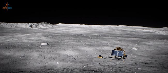
Chandrayaan-2 was launched on 22 July 2019. After achieving a 100 km (62 mile) circular polar orbit around the Moon, a lander module will separate from the orbiting spacecraft and descend to the lunar surface for a soft landing, which currently is expected to occur in September 2019, after a seven-week journey to the Moon. The target landing area is in the Moon’s southern polar region, where no lunar lander has operated before. A small rover vehicle will be deployed from the lander to conduct a 14-day mission on the lunar surface. The orbiting spacecraft is designed to conduct a one-year mapping mission.
Artist’s illustration of India’s lunar lander and the small rover vehicle on the surface of the moon. Source: ISRO
The launch vehicle
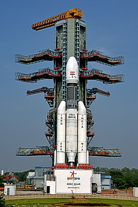
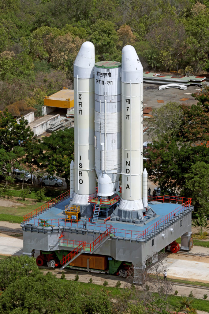
India will launch Chandrayaan-2 using the medium-lift Geosynchronous Satellite Launch Vehicle Mark III (GSLV Mk III) developed and manufactured by ISRO. As its name implies, GSLV Mk III was developed primarily to launch communication satellites into geostationary orbit. Variants of this launch vehicle also are used for science missions and a human-rated version is being developed to serve as the launch vehicle for the Indian Human Spaceflight Program.
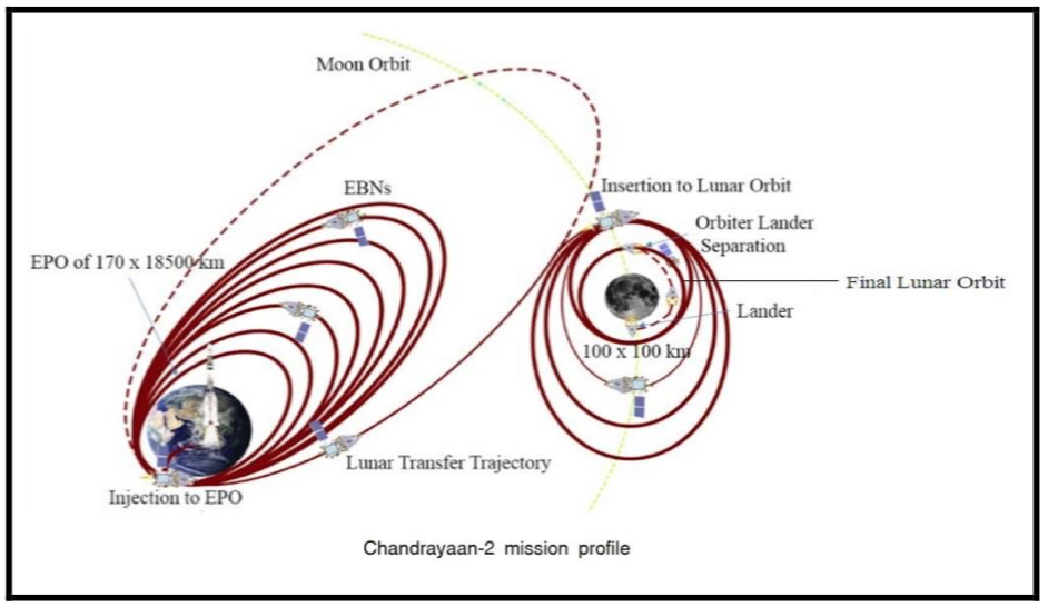
The GSLV III launch vehicle will place the Chandrayaan-2 spacecraft into an elliptical parking orbit (EPO) from which the spacecraft will execute orbital transfer maneuvers comparable to those successfully executed by Chandrayaan-1 on its way to lunar orbit in 2008. The Chandrayaan-2 mission profile is shown in the following graphic. You’ll find more information on the GSLV Mk III on the ISRO website at the following link: https://www.isro.gov.in/launchers/gslv-mk-iii
Source: ISRO
GSLV Mk III D2 on the launch pad at SDSC for the launchof the GSAT-29 communications satellite in 2018.Source: ISRO via Wikipedia
GSLV Mk III D1 lifting off from the SDSCwith the GSAT-19 communications satellite in 2017.Source: ISRO via WikipediaTransporting the partially integrated GSLV MkIII M1 launch vehicle for the Chandrayaan-2 mission on the Mobile Launch Pedestal. Source: ISRO
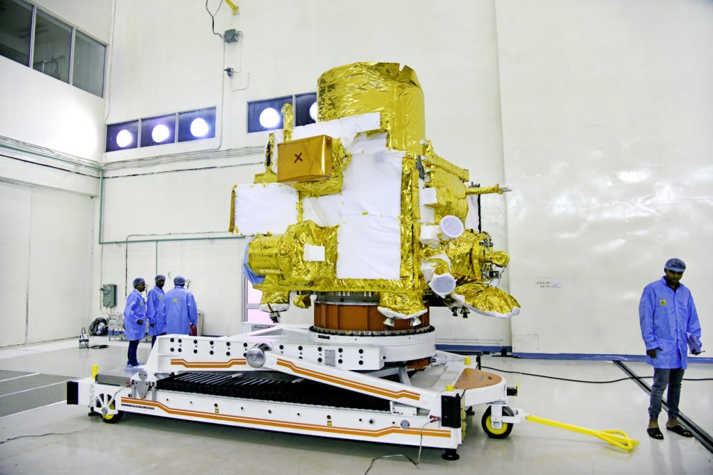
The spacecraft
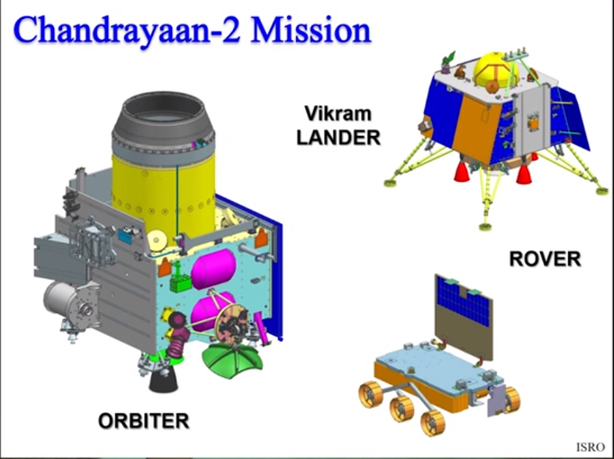
Chandrayaan-2 builds on the design and operating experience from the previous Chandrayaan-1 mission. The new spacecraft developed by ISRO has an initial mass of 3,877 kg (8,547 lb). It consists of three modules: an Orbiter Craft (OC) module, the Vikram Lander Craft (LC) module, and the small Pragyan rover vehicle, which is carried by the LC. The three modules are shown in the following diagram.
Three spacecraft modules (not to scale). Source: ISRO
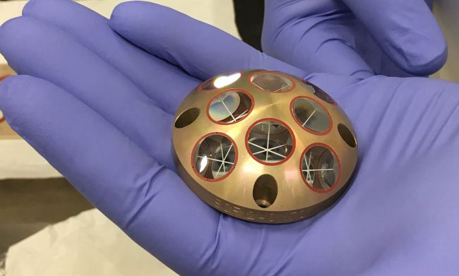
Chandrayaan-2 carries 13 Indian payloads — eight on the orbiter, three on the lander and two on the rover. In addition, the lander carries a passive Laser Retroreflector Array (LRA) provided by NASA.
Laser Retroreflector Array (LRA). Source: ISRO
The OC and the LC are stacked together within the payload fairing of the launch vehicle and remain stacked until the LC separates in lunar orbit and starts its descent to the lunar surface.
Orbiter (bottom) & lander (top) in stacked configuration. Source: ISRO
The solar-powered orbiter is designed for a one-year mission to map lunar surface characteristics (chemical, mineralogical, topographical), probe the lunar surface for water ice, and map the lunar exosphere using the CHACE-2 mass spectrometer. The orbiter also will relay communication between Earth and Vikram lander.
The orbiter. Source: ISRO
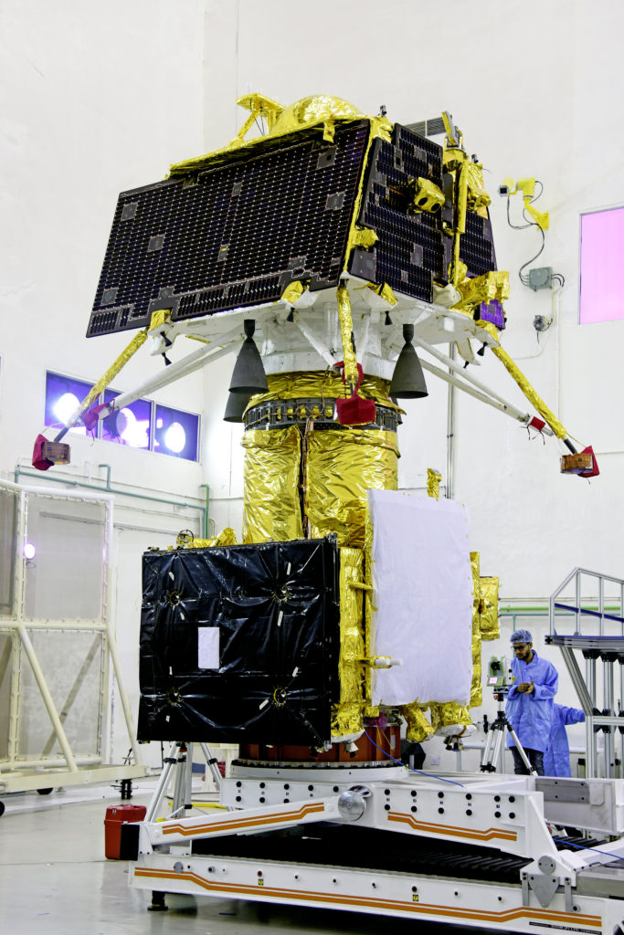
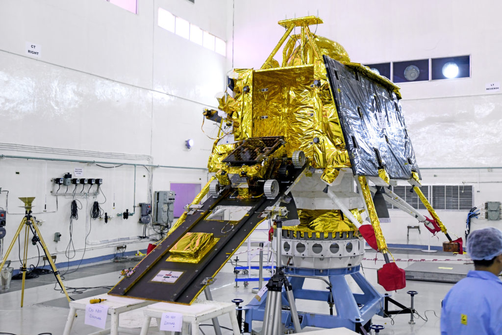
The solar-powered Vikram lander weighs 1,471 kg (3,243 lb). The scientific instruments on the lander will measure lunar seismicity, measure thermal properties of the lunar regolith in the polar region, and measure near-surface plasma density and its changes with time.
The Vikram lander with the Pragyan rover on the ramp.Source: ISRO
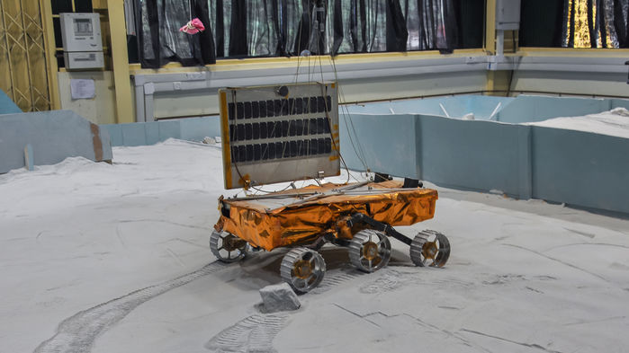
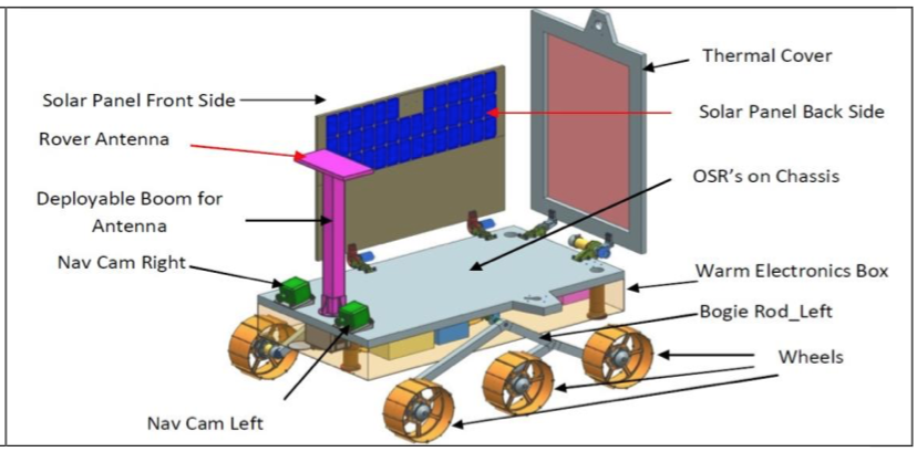
The 27 kg (59.5 lb) six-wheeled Pragyan rover, whose name means “wisdom” in Sanskrit, is solar-powered and capable of traveling up to 500 meters (1,640 feet) on the lunar surface. The rover can communicate only with the Vikram lander. It is designed for a 14-day mission on the lunar surface. It is equipped with cameras and two spectroscopes to study the elemental composition of lunar soil.
Rover during testing. Source: ISRORover details. Source: ISRO
You’ll find more information on the spacecraft in the 2018 article by V. Sundararajan, “Overview and Technical Architecture of India’s Chandrayaan-2 Mission to the Moon,” at the following link:
Best wishes to the Chandrayaan-2 mission team for a successful soft lunar landing and long-term lunar mapping mission.
Update 2 December 2019: Vikram lander crashed on the Moon
After a 48-day transit following launch, and an apparently nominal descent toward the lunar surface, communications with the Vikram lander were lost on 6 September 2019, when the spacecraft was at an altitude of about 2 km (1.2 miles), with just seconds remaining before the planned landing. Communications with the Chandrayaan orbiter continued after communications was lost with the Vikram lander. More details on India’s failed landing attempt are in the 25 November 2019 article on the Space.com website here: https://www.space.com/india-admits-moon-lander-crash.html
When charged molecules in the air are subjected to an electric field, they are accelerated. When these charged molecules collide with neutral ones, they transfer part of their momentum, leading to air movement known as an “ionic wind.” This basic process is shown in the following diagram, which depicts a strong electric field between a discharge electrode (left) and a ground electrode (right), and the motion of negative ions toward the ground electrode where they are collected. The neutral molecules pass through the ground electrode and generate the thrust called the ionic wind.
This post summarizes work that has been done to develop ionic wind propulsion systems for aircraft. The particular projects summarized are the following:
Major Alexander de Seversky’s Ionocraft vertical lifter (1964)
Michael Walden / LTAS lighter-than-air XEM-1 (1977)
Michael Walden / LTAS lighter-than-air EK-1 (2003)
The Festo b-IONIC Airfish airship (2005)
NASA ionic wind study (2009)
The MIT electroaerodynamic (EAD) heaver-than-air, fixed wing aircraft (2018)
In addition, we’ll take a look at recent ionic propulsion work being done by Electrofluidsystems Ltd., Electron Air LLC and the University of Florida’s Applied Physics Research Group.
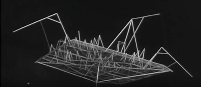
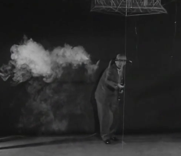
2. Scale model of ion-propelled Ionocraft vertical takeoff lifter flew in 1964
Major Alexander de Seversky developed the design concept for a novel aircraft concept called the “Ionocraft,” which was capable of hovering or moving in any direction at high altitudes by means of ionic discharge. His design for the Ionocraft is described in US Patent 3,130,945, “Ionocraft,” dated 28 April 1964. You can read this patent here: https://patents.google.com/patent/US3130945A/en
The operating principle of de Seversky’s Ionocraft propulsion system is depicted in the following graphic.
Ion propulsion scheme implemented in the de Seversky Ionocraft. Source: Popular Mechanics, August 1964
In 1964, de Seversky built a two-ounce (57 gram) Ionocraft scale model and demonstrated its ability to fly while powered from an external 90 watt power conversion system (30,000 volts at 3 mA), significantly higher that conventional aircraft and helicopters. This translated into a power-to-weight ratio of about 0.96 hp/pound. You can watch a short 1964 video of a scale model Ionocraft test flight here:
Screenshot showing Ionocraft scale model in flightScreenshot showing ionic wind downdraft under an Ionocraft scale model in flight
Alexander de Seversky’s one-man Ionocraft concept. Source: Popular Mechanics Archive, August 1964Alexander de Seversky’s Ionocraft commuter concept. Source: Popular Mechanics Archive, August 19641969 Soviet concepts for passenger carrying Ionocraft. Technology for Youth magazine, 1969, Issue 7.
In the 1960s, engineers found that Ionocraft technology did not scale up well and they were unable to build a vehicle that could generate enough lift to carry the equipment needed to produce the electricity needed to drive it.
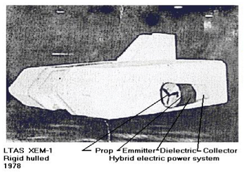
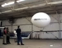
3. The first free-flying, ion-propelled, lighter-than-air craft flew in 1977: Michael Walden / LTAS XEM-1
The subscale XEM-1 proof-of-concept demonstrator was designed by Michael Walden and built in 1974 by his firm, Lighter Than Air Solar (LTAS) in Nevada. After leaving LTAS in 2005, Michael Walden founded Walden Aerospace where he is the President and CTO, building on the creative legacy of his work with the former LTAS firms. The Walden Aerospace website is here: http://walden-aerospace.com/HOME.html
The basic configuration of this small airship is shown in the following photo. The MK-1 ionic airflow (IAF) hybrid EK drives are mounted on the sides of the airship’s rigid hull.
Source: Walden Aerospace.
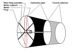
Basic configuration of the MK-1 ionic airflow (IAF) hybrid EK drive. Source: Walden Aerospace.
XEM-1 originally was tethered by cable to an external control unit and later was modified for wireless remote control operation. In this latter configuration, XEM-1 demonstrated the use of a hybrid EK propulsion system in a self-powered, free-flying vehicle.
Walden described the MK-1 IAF EK drive as follows: “The duct included a 10 inch ‘bent tip’ 3-bladed prop running on an electric motor to create higher pressures through the duct, making it a ‘modified pressure lifter’…. The duct also had a circular wire emitter, a dielectric separator and a toroidal collector making it a ‘toroid lifter’.”
The later MK-2 and MK-3 IAF EK drives had a similar duct configuration. In all of these EK drives, the flow of ions from emitter to collector imparts momentum to neutral air molecules, creating usable thrust for propulsion. You’ll find more information on the MK-1 IAF EK drive and later versions on the Walden Aerospace website here: http://walden-aerospace.com/Waldens_Patents_files/Walden%20Aerospace%20Advanced%20Technologies%2011092013-2.pdf
The XEM-1 was demonstrated to the Department of Defense (DoD) and Department of Energy (DOE) in 1977 at Nellis Air Force Base in Nevada. Walden reported: “We flew the first fully solar powered rigid airship in 1974, followed by a US Department of Defense and Department of Energy flight demonstration in August 1977”…. “ DoD was interested in this work to the extent that some of it is still classified despite requests for the information to become freely available.”
Walden credits the XEM-1 with being the first fully self-contained air vehicle to fly with a hybrid ionic airflow electro-kinetic propulsion system. This small airship also demonstrated the feasibility of a rigid, composite, monocoque aeroshell, which became a common feature on many later Walden / LTAS airships.
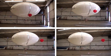
4. The second free-flying, ion-propelled, lighter-than-air craft flew in 2003: Michael Walden / LTAS EK-1
Michael Walden designed the next-generation EK-1, which was a remotely controlled, self-powered, subscale model of a lenticular airship with a skin-integrated EK drive that was part of the outer surface of the hull. The drive was electronically steered to provide propulsion in any direction with no external aerodynamic surfaces and no moving parts.
EK-1 aloft in the hanger. Source: LTAS / Walden Aerospace
EK-1 with a skin-integrated propulsion system moving during hanger test flight in 2003.Source: LTAS / Walden Aerospace
In June 2003, LTAS rented a hangar at the Boulder City, NV airport to build and fly the EK-1. Testing the EK-1 was concluded in early August 2003 after demonstrating the technology to National Institute for Discovery Science (NIDS) board members.
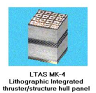
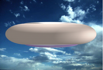
Based on the EK-1 design, a full-scale EK airship would have a rigid, aeroshell comprised largely of LTAS MK-4 lithographic integrated thruster / structure hull panels. As with other contemporary Walden / LTAS airship designs, the MK-4 panel airship likely would have implemented density controlled buoyancy (DCB) active aerostatic lift control and would have had a thin film solar array on the top of the aeroshell.
Artist’s concept of a MK-4 panel airship. Source: Walden Aerospace
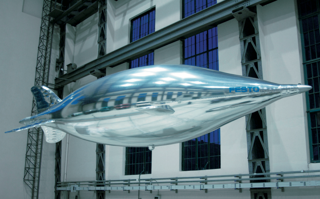
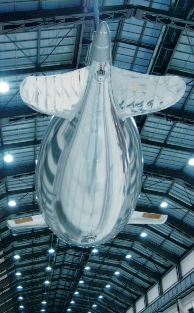
5. The third free-flying, ion-propelled, lighter-than-air craft flew in 2005: the Festo b-IONIC Airfish
The Festo b-IONIC Airfish airship was developed at the Technical University of Berlinwith guidance of the firm Festo AG & Co. KG. This small, non-rigid airship is notable because, in 2005, it became the first aircraft to fly with a solid state propulsion system. The neutrally-buoyant Airfish only flew indoors, in a controlled environment, at a very slow speed, but it flew.
Airfish. Source: Festo AG & Co. KG
Some of the technical characteristics of the Airfish are listed below:
Length: 7.5 meters (24.6 ft)
Span: 3.0 meters (9.8 ft)
Shell diameter: 1.83 meters (6 ft)
Helium volume: 9.0 m3(318 ft3)
Total weight: 9.04 kg (19.9 lb)
Power source in tail: 12 x 1,500 mAh lithium-ion polymer cells (18 Ah total)
Power source per wing (two wings): 9 x 3,200 mAh lithium-ion polymer cells (28.8 Ah total)
High voltage: 20,000 to 30,000 volts
Buoyancy: 9.0 – 9.3 kg (19.8 – 20.5 lb)
Total thrust: 8 – 10 grams (0.018 – 0.022 pounds)
Maximum velocity: 0.7 meters/sec (2.5 kph; 1.6 mph)
The b-IONIC Airfish employed two solid state propulsion systems, an electrostatic ionic jet and a plasma ray, which Festo describes as follows:
Electrostatic ionic jet: “At the tail end Airfish uses the classic principle of an electrostatic ionic jet propulsion engine. High-voltage DC-fields (20-30 kV) along thin copper wires tear electrons away from air molecules. The positive ions thus created are then accelerated towards the negatively charged counter electrodes (ring-shaped aluminum foils) at high speeds (300-400 m/s), pulling along additional neutral air molecules. This creates an effective ion stream with speeds of up to 10 m/s.”
Plasma-ray: “The side wings of Airfish are equipped with a new bionic plasma-ray propulsion system, which mimics the wing based stroke principle used by birds, such as penguins, without actually applying movable mechanical parts. As is the case with the natural role model, the plasma-ray system accelerates air in a wavelike pattern while it is moving across the wings.”
Airfish. Source: Festo AG & Co. KG
Airfish. Source: Festo AG & Co
The Festo b-IONIC Airfish demonstrated that a solid state propulsion system was possible. The tests also demonstrated that the solid state propulsion systems also reduced drag, raising the intriguing possibility that it may be possible to significantly reduce drag if an entire vessel could be enclosed in a ionized plasma bubble.You’ll find more information on the Festo b-IONIC Airfish, its solid state propulsion system and implications for drag reduction in the the Festo brochure here: https://www.festo.com/net/SupportPortal/Files/344798/b_IONIC_Airfish_en.pdf
You can watch a 2005 short video on the Festo b-IONIC Airfish flight here:
6. NASA ionic wind study – 2009
A corona discharge device generates an ionic wind, and thrust, when a high voltage corona discharge is struck between sharply pointed electrodes and larger radius ground electrodes.
In 2009, National Aeronautics & Space Administration (NASA) researchers Jack Wilson, Hugh Perkins and William Thompson conducted a study to examine whether the thrust of corona discharge systems could be scaled to values of interest for aircraft propulsion. Their results are reported in report NASA/TM-2009-215822, which you’ll find at the following link: https://ntrs.nasa.gov/archive/nasa/casi.ntrs.nasa.gov/20100000021.pdf
Key points of the study included:
Different types of high voltage electrodes were tried, including wires, knife-edges, and arrays of pins. A pin array was found to be optimum.
Parametric experiments, and theory, showed that the thrust per unit power could be raised from early values of 5 N/kW to values approaching 50 N/kW, but only by lowering the thrust produced, and raising the voltage applied.
In addition to using DC voltage, pulsed excitation, with and without a DC bias, was examined. The results were inconclusive as to whether this was advantageous.
It was concluded that the use of a corona discharge for aircraft propulsion did not seem very practical.”
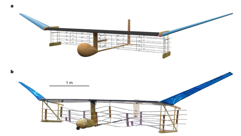
7. The first heavier-than-air, fixed-wing, ion-propelled aircraft flew in 2018
On 21 November 2018, MIT researchers reported successfully flying the world’s first heavier-than-air, fixed-wing, ion-propelled (electroaerodynamic, EAD) aircraft. You can read the paper by Haofeng Xu, et al., “Flight of an aeroplane with solid-state propulsion,” on the Nature website here: https://www.nature.com/articles/s41586-018-0707-9
The design of the MIT EAD aircraft is shown below:
a, Computer-generated rendering of the EAD airplane. b, Photograph of actual EAD airplane (after multiple flight trials).
Some of the technical characteristics of this MIT aircraft are listed below:
Wingspan: 4.9 meters (16 ft)
Total weight: 2.45 kg (5.4 lb)
Power source: powered by 54 x 3.7 volt 150 mAh lithium-ion polymer cells (8.1 Ah total)
Maximum velocity: 4.8 meters/sec (17.3 kph; 10.7 mph)
In their paper, the MIT researchers reported:
“We performed ten flights with the full-scale experimental aircraft at the MIT Johnson Indoor Track…. Owing to the limited length of the indoor space (60 m), we used a bungeed launch system to accelerate the aircraft from stationary to a steady flight velocity of 5 meters/sec within 5 meters, and performed free flight in the remaining 55 meters of flight space. We also performed ten unpowered glides with the thrusters turned off, in which the airplane flew for less than 10 meters. We used cameras and a computer vision algorithm to track the aircraft position and determine the flight trajectory.”
“All flights gained height over the 8–9 second segment of steady flight, which covered a distance of 40–45 meters…. The average physical height gain of all flights was 0.47 meters…. However, for some of the flights, the aircraft velocity decreased during the flight. An adjustment for this loss of kinetic energy…. results in an energy equivalent height gain, which is the height gain that would have been achieved had the velocity remained constant. This was positive for seven of the ten flights, showing that better than steady-level flight had been achieved in those cases.”
“In this proof of concept for this method of propulsion, the realized thrust-to-power ratio was 5 N/kW1, which is of the order of conventional airplane propulsion methods such as the jet engine.” Overall efficiency was estimated to be 2.56%.
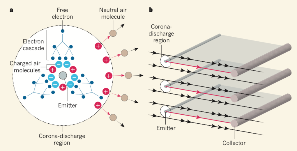
The propulsion principles of the MIT EAD aircraft are explained in relation to the following diagram in the November 2018 article by Franck Plouraboué, “Flying With Ionic Wind,” which you can read on the Nature website at the following link: https://www.nature.com/articles/d41586-018-07411-z
The following diagram and explanatory text are reproduced from that article.
In Figure a, above: …an electric field (not shown) is applied to the region surrounding a fine wire called the emitter (shown in cross-section). The field induces electron cascades, whereby free electrons collide with air molecules (not shown in the cascades) and consequently free up more electrons. This process produces charged air molecules in the vicinity of the emitter — a corona discharge. Depending on the electric field, negatively or positively charged molecules drift away (red arrows) from the emitter. These molecules collide with neutral air molecules, generating an ionic wind (black arrows).
In Figure b, above: The aircraft uses a series of emitters and devices called collectors, the longitudinal directions of which are perpendicular to the ionic wind. The flow of charged air molecules occurs mainly along the directions (red arrows) joining emitters and collectors. Consequently, the ionic wind is accelerated (black arrows) predominantly in these regions.
You can view a short video of the MIT EAD aircraft test flights here:
8. The future of ionic propulsion for aerospace applications.
If it can be successfully developed to much larger scales, ionic propulsion offers the potential for aircraft to fly in the atmosphere on a variety of practical missions using only ionized air for propulsion. Using other ionized fluid media, ionic propulsion could develop into a means to fly directly from the surface of the earth into the vacuum of space and then operate in that environment. The following organizations have been developing such systems.
Electrofluidsystems Ltd.
In 2006, the Technical University of Berlin’s Airfish project manager, Berkant Göksel, founded the firm Electrofluidsystems Ltd., which in 2012 was rebranded as IB Göksel Electrofluidsystems. This firm presently is developing a new third generation of plasma-driven airships with highly reduced ozone and nitrogen oxide (NOx) emissions, magneto-plasma actuators for plasma flow control, and the company’s own blended wing type flying wing products. You’ll find their website here: https://www.electrofluidsystems.com
Source: Electrofluidsystems TU BerlinAdvanced plasma-driven aircraft concept. Source: Electrofluidsystems TU Berlin
MIT researchers are developing designs for high-performance aircraft using ionic propulsion. Theoretically, efficiency improves with speed, with an efficiency of 50% possible at a speed of about 1,000 kph (621 mph). You can watch a short video on MIT work to develop a Star Trek-like ion drive aircraft here:
Electron Air LLC
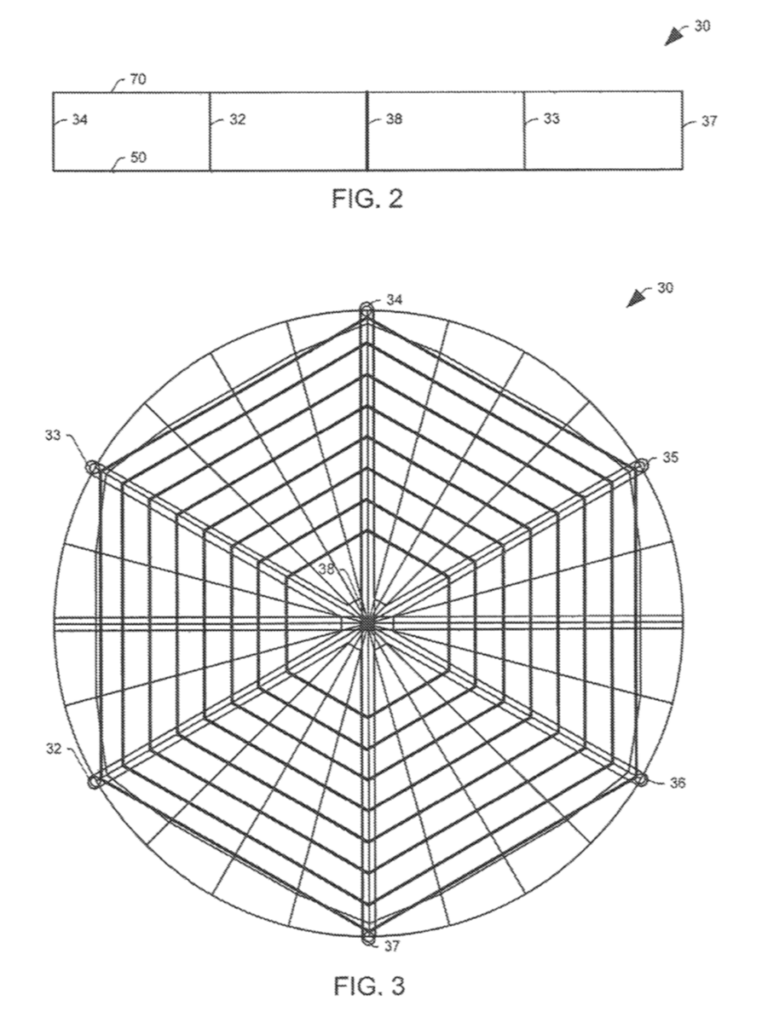
Another firm active in the field of ionic propulsion is Electron Air LLC (https://electronairllc.org), which, on 6 November 2018, was granted patent US10119527B2 for their design for a self-contained ion powered craft. Their grid shaped craft is described as follows:
“The aircraft assembly includes a collector assembly, an emitter assembly, and a control circuit operatively connected to at least the emitter and collector assemblies and comprising a power supply configured to provide voltage to the emitter and collector assemblies. The assembly is configured, such that, when the voltage is provided from an on board power supply, the aircraft provides sufficient thrust to lift each of the collector assembly, the emitter assembly, and the entire power supply against gravity.”
The device, as shown in patent Figure 3, consists of a two-layer grid structure with a collector assembly (50), an emitter assembly (70) and peripheral supports (33 to 37).
This patent cites Alexander de Seversky’s Patent 3130945, “Ionocraft.”
You can watch a short (1:22 minute) video of an outdoor tethered test flight of a remotely controlled, self-contained, ion powered, heavier-than-air craft with onboard power at the following link: https://www.youtube.com/watch?v=aX21HCHlgKo
University of Florida, Applied Physics Research Group
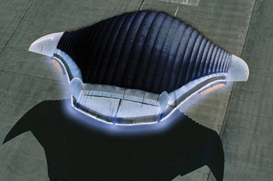
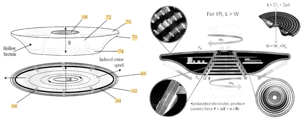
In the early 2000s, a Wingless Electromagnetic Air Vehicle (WEAV) was invented by Dr. Subrata Roy, a plasma physicist and aerospace engineering professor at the University of Florida. WEAV is described as a heavier-than-air flight system that can self-lift, hover, and fly using plasma propulsion with no moving components. The laboratory-scale device is six inch (15.2 cm) in diameter. The basic configuration of the disc-shaped craft is shown in patent 8960595B2 Figure 1.
This research project has been supported by the US Air Force Office of Scientific Research. You’ll find details on WEAV technology in the University of Florida’s 2011 final report at the following (very slow loading) link:https://apps.dtic.mil/dtic/tr/fulltext/u2/a564120.pdf
In this report, the authors describe the technology: “This revolutionary concept is based on the use of an electro-(or magneto) hydrodynamic (EHD/MHD) thrust generation surface that is coated with multiple layers of dielectric polymers with exposed and/or embedded electrodes for propulsion and dynamic control. This technology has the unique capability of imparting an accurate amount of thrust into the surrounding fluid enabling the vehicle to move and react. Thrust is instantaneously and accurately controlled by the applied power, its waveform, duty cycle, phase lag and other electrical parameters. Once the applied power is removed the thrust vanishes.”
The following patents related to WEAV technology have been filed and assigned to the University of Florida Research Foundation Inc.:
M. Robinson, “Movement of Air in the Electric Wind of the Corona Discharge:, Technical Paper TP60-2, Research-Cottrell, Inc., Bound Brook, NJ, 8 June 1960; https://apps.dtic.mil/dtic/tr/fulltext/u2/262830.pdf
P. Zheng, et al., “A Comprehensive Review of Atmospheric-Breathing Electric Propulsion Systems,” International Journal of Aerospace Engineering, Article ID 8811847, 7 October 2020; https://www.hindawi.com/journals/ijae/2020/8811847/
Nicolas Monrolin, Franck Plouraboué, Olivier Praud.“Electrohydrodynamic Thrust for In-Atmosphere Propulsion,” AIAA Journal, American Institute of Aeronautics and Astronautics, 2017, vol. 55 (n° 12), pp. 4296-4305. 10.2514/1.J055928 . hal-01660600; https://hal.archives-ouvertes.fr/hal-01660600/document
Daniel Drew, “The Ionocraft: Flying Microrobots With No Moving Parts,” Technical Report No. UCB/EECS-2018-164, Electrical Engineering and Computer Sciences, University of California at Berkeley, 10 December 2018; https://www2.eecs.berkeley.edu/Pubs/TechRpts/2018/EECS-2018-164.pdf
WEAV
Subrata Roy, et al., “Demonstration of a Wingless Electromagnetic Air Vehicle,” Final Report AFRL-OSR-VA-TR-2012-0922, University of Florida, Applied Physics Research Group: https://apps.dtic.mil/dtic/tr/fulltext/u2/a564120.pdf
1. Overview of US military optical reconnaissance satellite programs
The National Reconnaissance Office (NRO) is responsible for developing and operating space reconnaissance systems and conducting intelligence-related activities for US national security. NRO developed several generations of classified Keyhole (KH) military optical reconnaissance satellites that have been the primary sources of Earth imagery for the US Department of Defense (DoD) and intelligence agencies. NRO’s website is here:
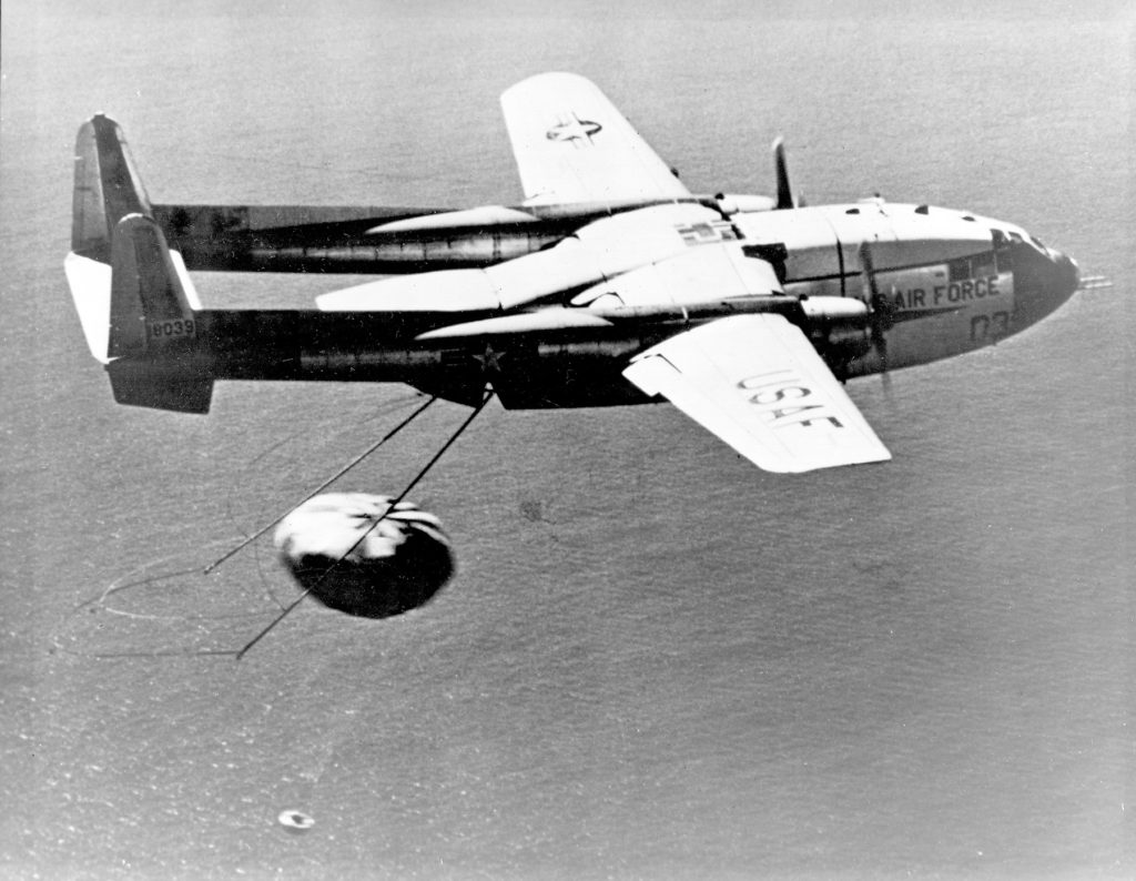
NRO’s early generations of Keyhole satellites were placed in low Earth orbits, acquired the desired photographic images on film during relatively short-duration missions, and then returned the film to Earth in small reentry capsules for airborne recovery. After recovery, the film was processed and analyzed. The first US military optical reconnaissance satellite program, code named CORONA, pioneered the development and refinement of the technologies, equipment and systems needed to deploy an operational orbital optical reconnaissance capability. The first successful CORONA film recovery occurred on 19 August 1960.
Specially modified US Air Force C-119J aircraft recovers a CORONA film canister in flight. Source: US Air Force
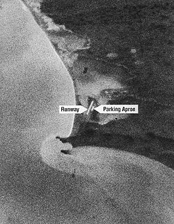
First reconnaissance picture taken in orbit and successfully recovered on Earth; taken on 18 August 1960 by a CORONA KH-1 satellite dubbed Discoverer 14. Image shows the Mys Shmidta airfield in the Chukotka region of the Russian Arctic, with a resolution of about 40 feet (12.2 meters). Source: Wikipedia
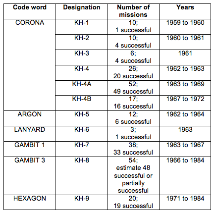
Keyhole satellites are identified by a code word and a “KH” designator, as summarized in the following table.
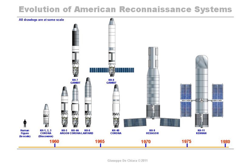
In 1976, NRO deployed its first electronic imaging optical reconnaissance satellite known as KENNEN KH-11 (renamed CRYSTAL in 1982), which eventually replaced the KH-9, and brought an end to reconnaissance satellite missions requiring film return. The KH-11 flies long-duration missions and returns its digital images in near real time to ground stations for processing and analysis. The KH-11, or an advanced version sometimes referred to as the KH-12, is operational today.
US film-return reconnaissance satellites from KH-1 to KH-9 shown to scale with the KH-11 electronic imaging reconaissance satellite. Credit: Giuseppe De Chiara and The Space Review.
Geospatial intelligence, or GEOINT, is the exploitation and analysis of imagery and geospatial information to describe, assess and visually depict physical features and geographically referenced activities on the Earth. GEOINT consists of imagery, imagery intelligence and geospatial information. Satellite imagery from Keyhole reconnaissance satellites is an important information source for national security-related GEOINT activities.
The National Geospatial-Intelligence Agency (NGA), which was formed in 2003, has the primary mission of collecting, analyzing, and distributing GEOINT in support of national security. NGA’s predecessor agencies, with comparable missions, were:
National Imagery and Mapping Agency (NIMA), 1996 – 2003
National Photographic Interpretation Center (NPIC), a joint project of the Central Intelligence Agency (CIA) and DoD, 1961 – 1996
2. The advent of the US civilian Earth observation programs
Collecting Earth imagery from orbit became an operational US military capability more than a decade before the start of the joint National Aeronautics & Space Administration (NASA) / US Geological Survey (USGS) civilian Landsat Earth observation program. The first Landsat satellite was launched on 23 July 1972 with two electronic observing systems, both of which had a spatial resolution of about 80 meters (262 feet).
Since 1972, Landsat satellites have continuously acquired low-to-moderate resolution digital images of the Earth’s land surface, providing long-term data about the status of natural resources and the environment. Resolution of the current generation multi-spectral scanner on Landsat 9 is 30 meters (98 feet) in visible light bands.
3. Declassification of certain military reconnaissance satellite imagery
All military reconnaissance satellite imagery was highly classified until 1995, when some imagery from early defense reconnaissance satellite programs was declassified. The USGS explains:
“The images were originally used for reconnaissance and to produce maps for U.S. intelligence agencies. In 1992, an Environmental Task Force evaluated the application of early satellite data for environmental studies. Since the CORONA, ARGON, and LANYARD data were no longer critical to national security and could be of historical value for global change research, the images were declassified by Executive Order 12951 in 1995”
Additional sets of military reconnaissance satellite imagery were declassified in 2002 and 2011 based on extensions of Executive Order 12951.
The declassified imagery is held by the following two organizations:
The original film is held by the National Archives and Records Administration (NARA).
Duplicate film held in the USGS Earth Resources Observation and Science (EROS) Center archive is used to produce digital copies of the imagery for distribution to users.
The declassified military satellite imagery available in the EROS archive is summarized below:
USGS EROS Archive – Declassified Satellite Imagery – 1 (1960 to 1972)
This set of photos, declassified in 1995, consists of more than 860,000 images of the Earth’s surface from the CORONA, ARGON, and LANYARD satellite systems.
CORONA image resolution improved from 40 feet (12.2 meters) for the KH-1 to about 6 feet (1.8 meters) for the KH-4B.
KH-5 ARGON image resolution was about 460 feet (140 meters).
KH-6 LANYARD image resolution was about 6 feet (1.8 meters).
USGS EROS Archive – Declassified Satellite Imagery – 2 (1963 to 1980)
This set of photos, declassified in 2002, consists of photographs from the KH-7 GAMBIT surveillance system and KH-9 HEXAGON mapping program.
KH-7 image resolution is 2 to 4 feet (0.6 to 1.2 meters). About 18,000 black-and-white images and 230 color images are available.
The KH-9 mapping camera was designed to support mapping requirements and exact positioning of geographical points. Not all KH-9 satellite missions included a mapping camera. Image resolution is 20 to 30 feet (6 to 9 meters); significantly better than the 98 feet (30 meter) resolution of LANDSAT imagery. About 29,000 mapping images are available.
USGS EROS Archive – Declassified Satellite Imagery – 3 (1971 to 1984)
This set of photos, declassified in 2011, consists of more photographs from the KH-9 HEXAGON mapping program. Image resolution is 20 to 30 feet (6 to 9 meters).
4. Example applications of declassified military reconnaissance satellite imagery
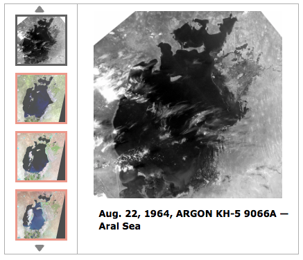
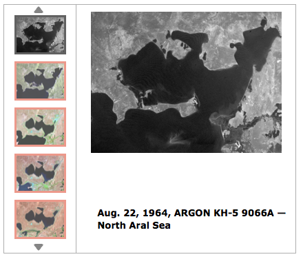
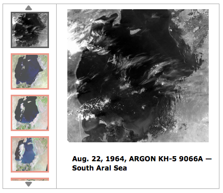
The declassified military reconnaissance satellite imagery provides views of the Earth starting in the early 1960s, more than a decade before civilian Earth observation satellites became operational. The military reconnaissance satellite imagery, except from ARGON KH-5, is higher resolution than is available today from Landsat civilian earth observation satellites. The declassified imagery is an important supplement to other Earth imagery sources. Several examples applications of the declassified imagery are described below.
4.1 Assessing Aral Sea depletion
USGS reports: “The Aral Sea once covered about 68,000 square kilometers, a little bigger than the U.S. state of West Virginia. It was the 4th largest lake in the world. It is now only about 10% of the size it was in 1960…..In the 1990s, a dam was built to prevent North Aral water from flowing into the South Aral. It was rebuilt in 2005 and named the Kok-Aral Dam…..The North Aral has stabilized but the South Aral has continued to shrink and become saltier. Up until the 1960s, Aral Sea salinity was around 10 grams per liter, less than one-third the salinity of the ocean. The salinity level now exceeds 100 grams per liter in the South Aral, which is about three times saltier than the ocean.”
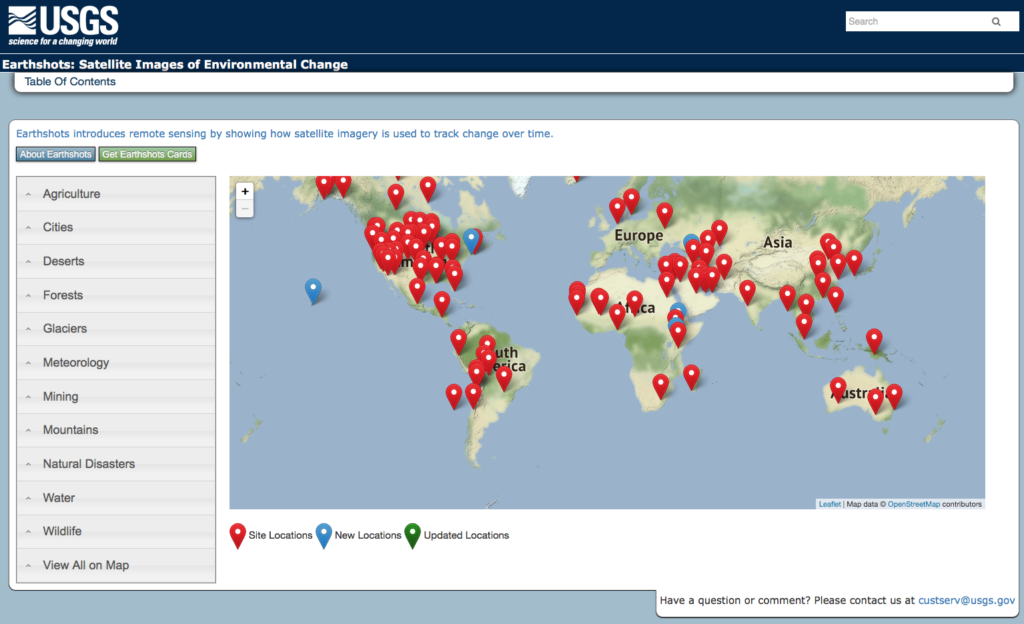
On the USGS website, the “Earthshots: Satellite Images of Environmental Change” webpages show the visible changes at many locations on Earth over a 50+ year time period. The table of contents to the Earthshots webpages is shown below and is at the following link: http:// https://earthshots.usgs.gov/earthshots/
USGS Earthshots Table of Contents
For the Aral Sea region, the Earthshots photo sequences start with ARGON KH-5 photos taken in 1964. Below are three screenshots of the USGS Earthshots pages showing the KH-5 images for the whole the Aral Sea, the North Aral Sea region and the South Aral Sea region. You can explore the Aral Sea Earthshots photo sequences at the following link: https://earthshots.usgs.gov/earthshots/node/91#ad-image-0-0
4.2 Assessing Antarctic ice shelf condition
In a 7 June 2016 article entitled, ”Spy satellites reveal early start to Antarctic ice shelf collapse,” Thomas Sumner reported:
“Analyzing declassified images from spy satellites, researchers discovered that the downhill flow of ice on Antarctica’s Larsen B ice shelf was already accelerating as early as the 1960s and ’70s. By the late 1980s, the average ice velocity at the front of the shelf was around 20 percent faster than in the preceding decades,….”
Satellite images taken by the ARGON KH-5 satellite have revealed how the accelerated movement that triggered the collapse of the Larsen B ice shelf on the east side of the Antarctic Peninsula began in the 1960s. The declassified images taken by the satellite on 29 August 1963 and 1 September 1963 are pictured right. Source: Daily Mail, 10 June 2016
4.3 Assessing Himalayan glacier condition
In a 19 June 2019 paper “Acceleration of ice loss across the Himalayas over the past 40 years,” the authors, reported on the use of HEXAGON KH-9 mapping camera imagery to improve their understanding of trends affecting the Himalayan glaciers from 1975 to 2016:
“Himalayan glaciers supply meltwater to densely populated catchments in South Asia, and regional observations of glacier change over multiple decades are needed to understand climate drivers and assess resulting impacts on glacier-fed rivers. Here, we quantify changes in ice thickness during the intervals 1975–2000 and 2000–2016 across the Himalayas, using a set of digital elevation models derived from cold war–era spy satellite film and modern stereo satellite imagery.”
“The majority of the KH-9 images here were acquired within a 3-year interval (1973–1976), and we processed a total of 42 images to provide sufficient spatial coverage.”
“We observe consistent ice loss along the entire 2000-km transect for both intervals and find a doubling of the average loss rate during 2000–2016.”
“Our compilation includes glaciers comprising approximately 34% of the total glacierized area in the region, which represents roughly 55% of the total ice volume based on recent ice thickness estimates.”
3-D image of the Himalayas derived from HEXAGON KH-9 satellite mapping photographs taken on December 20, 1975.Source: J. M. Maurer/LDEO
4.4 Discovering archaeological sites
A. CORONA Atlas Project
The Center for Advanced Spatial Technologies, a University of Arkansas / U.S. Geological Survey collaboration, has undertaken the CORONA Atlas Project using military reconnaissance satellite imagery to create the “CORONA Atlas & Referencing System”. The current Atlas focuses on the Middle East and a small area of Peru, and is derived from 1,024 CORONA images taken on 50 missions. The Atlas contains 833 archaeological sites.
“In regions like the Middle East, CORONA imagery is particularly important for archaeology because urban development, agricultural intensification, and reservoir construction over the past several decades have obscured or destroyed countless archaeological sites and other ancient features such as roads and canals. These sites are often clearly visible on CORONA imagery, enabling researchers to map sites that have been lost and to discover many that have never before been documented. However, the unique imaging geometry of the CORONA satellite cameras, which produced long, narrow film strips, makes correcting spatial distortions in the images very challenging and has therefore limited their use by researchers.”
Screenshot of the CORONA Atlas showing regions in the Middle East with data available.
CAST reports that they have “developed methods for efficient
orthorectification of CORONA imagery and now provides free public access to our imagery database for non-commercial use. Images can be viewed online and full resolution images can be downloaded in NITF format.”
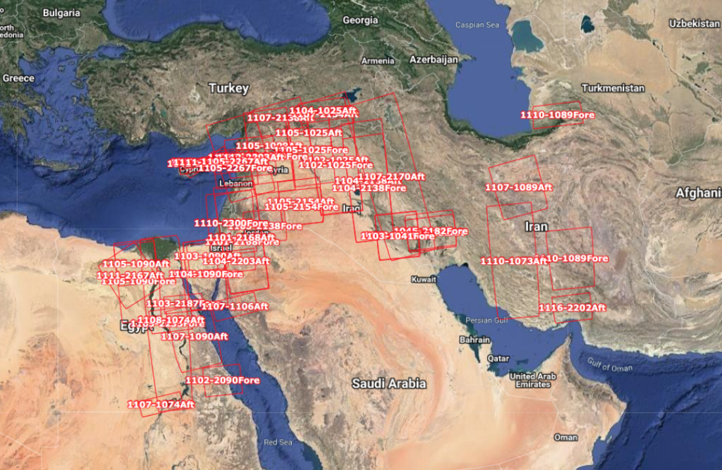
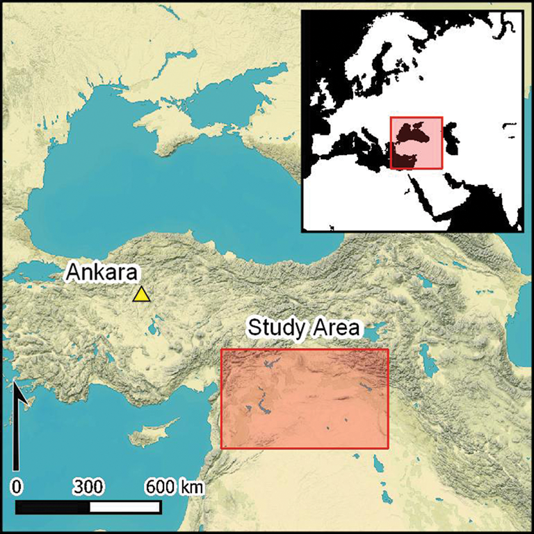
In October 2023, a team from Dartmouth College published a paper that described their recent discovery of 396 Roman-era forts using declassified CORONA and HEXAGON spy satellite imagery of regions of Syria, Iraq and nearby “fertile crescent” territories of the eastern Mediterranean. The study area is shown in the following map. A previous aerial survey of the area in 1934 had identified 116 other forts in the same region.
Dartmouth study area. Source: J. Casana, et al. (26 October 2023)
The authors noted, “Perhaps the most significant realization from our work concerns the spatial distribution of the forts across the landscape, as this has major implications for our understanding of their intended purpose as well as for the administration of the eastern Roman frontier more generally.”
Comparison of the distribution of forts documented in the 1934 aerial survey (top)and forts found recently on declassified satellite imagery (bottom).Source: Figure 9, J. Casana, et al. (26 October 2023)
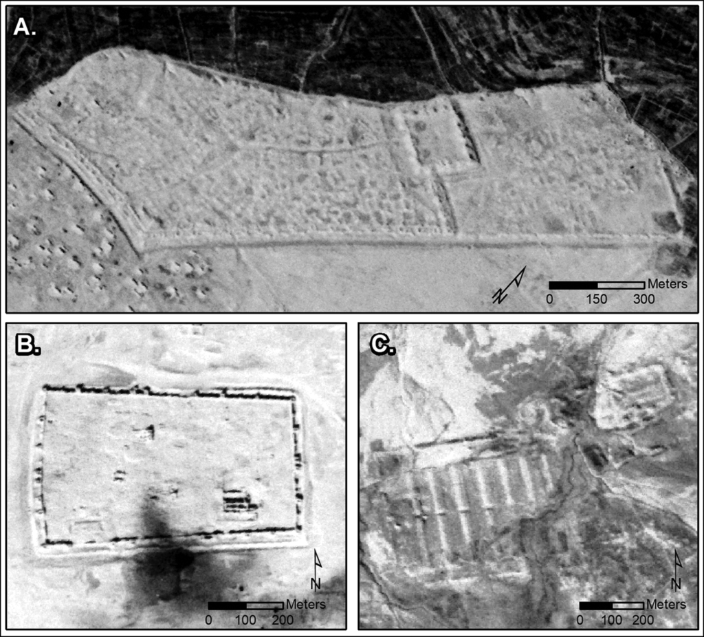
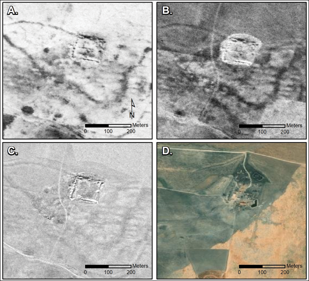
Examples of the new forts identified by the Dartmouth team in satellite imagery are shown in the following figures.
CORONA images showing three major sites: (A) Sura (NASA1401); (B) Resafa (NASA1398); and (C) Ain Sinu (CRN999).Source: Figure 3, J. Casana, et al. (26 October 2023)
Castellum at Tell Brak site in multiple images: (A) CORONA (1102, 17 December 1967); (B) CORONA (1105, 4 November 1968); (C) HEXAGON (1204, 17 November 1974); and (D) modern satellite imagery. Source: Figure 4, J. Casana, et al. (26 October 2023)
The teams paper concludes: “Finally, the discovery of such a large number of previously undocumented ancient forts in this well-studied region of the Near East is a testament to the power of remote-sensing technologies as transformative tools in contemporary archaeological research.”
4.5 Conducting commercial geospatial analytics over a broader period of time
The firm Orbital Insight, founded in 2013, is an example of commercial firms that are mining geospatial data and developing valuable information products for a wide range of customers. Orbital Insight reports:
“Orbital Insight turns millions of images into a big-picture understanding of Earth. Not only does this create unprecedented transparency, but it also empowers business and policy decision makers with new insights and unbiased knowledge of socio-economic trends. As the number of Earth-observing devices grows and their data output expands, Orbital Insight’s geospatial analytics platform finds observational truth in an interconnected world. We map out and quantify the world’s complexities so that organizations can make more informed decisions.”
“By applying artificial intelligence to satellite, UAV, and other geospatial data sources, we seek to discover and quantify societal and economic trends on Earth that are indistinguishable to the human eye. Combining this information with terrestrial data, such as mobile and location-based data, unlocks new sources of intelligence.”
5. Additional reading related to US optical reconnaissance satellites
You’ll find more information on the NRO’s film-return, optical reconnaissance satellites (KH-1 to KH-9) at the following links:
Robert Perry, “A History of Satellite Reconnaissance,” Volumes I to V, National Reconnaissance Office (NRO), various dates 1973 – 1974; released under FOIA and available for download on the NASA Spaceflight.com website, here: https://forum.nasaspaceflight.com/index.php?topic=20232.0
George Orwell’s novel Nineteen Eighty-Four was published 70 years ago, on 8 June 1949. Together with his political allegory Animal Farm published in 1945, Nineteen Eighty-Four brought Orwell worldwide fame. As I hope you know, Nineteen Eighty-Four describes a dystopian future occurring in 1984 (now 35 years in our past) in which a totalitarian government imposes repressive regimentation on all persons and behaviors through prescriptive laws, propaganda, manipulation of history, and omnipresent surveillance. Fortunately for us, the real year 1984 fared much better. However, Orwell’s vision of the future, as expressed in this novel, still may be a timely and cautionary tale of a future yet to come.
First edition cover. Source: Wikipedia
George Orwell. Source: BBC
You’ll find an interesting collection of quotations attributed to George Orwell on the AZ Quotes website here:
You can read Nineteen Eighty-Four chapter-by-chapter online on The Complete Works of George Orwell website at the following link, which also contains other Orwell novels.
Here, it’s easy to search the whole novel for key words and phrases, like “Though Police,” “Big Brother,” “Ministry of Truth,” “thoughtcrime,” “crimethink,” and “face crime,” and see how they are used in context.
Orwell was right about the concept that an entire population can be kept under constant surveillance. However, he probably didn’t appreciate the commercial value of such surveillance and that people voluntarily would surrender so much information into an insecure (online) environment, thereby making it easy for agents to legally or illicitly collect and process the information they want. Today, it’s hard to know if Big Brother is the government or anonymous aggregations of commercial firms seeking to derive value from your data and influence your behavior.
With the increasing polarization in our society today, it seems to me that we are entering more precarious times, where our own poorly defined terms, such as “politically correct” and “hate speech,” are becoming tools to stifle alternative views and legitimate dissent.
I remember in the late 1970s when I first read the words “politically correct” in Jim Holman’s local San Diego newspaper, Reader. My first reaction to this poorly defined term was that it will lead to no good. Since then, use of “politically correct” has grown dramatically, as shown in the following Google Ngram. While I agree that political correctness has its place in a polite society, the muddled jargon of political correctness easily can becomes a means to obfuscate a subject under discussion.
Ngram 1800 – 2008. Source: Google
In the past two decades, use of the term “hate speech” has become commonplace, as shown in the following Google Ngram. While laws have been written to define and combat actual “hate speech,” this term is easily misused to stifle dissent, even legitimate dissent, by forcefully mischaracterizing one side of a discussion that never was intended to be hateful. Our ability to hold opposing views without being mischaracterized as a “hater” is being eroded in our increasingly polarized society, where self-appointed (and often anonymous) Thought Police are using social media (What an oxymoron!) to punish the perceived offenders. Such “policing” is not centralized, as in Orwell’s novel, but its effects can be very damaging to its victims.
Ngram 1800 – 2008. Source: Google
Of course, the word “dissent” has been in common usage for a very long time and is a fundamental right of American citizens.
Ngram 1800 – 2008. Source: Google
Seventy years after first being published, Orwell’s novel Nineteen Eighty-Four still stands as a relevant cautionary tale for our own future. I encourage you to read it again, keep an open mind, and piss off the self-declared Thought Police from time to time.
Higgins landing craft are the ubiquitous, flat-bottomed, shallow-draft, barge-like boats used widely throughout WW II to deliver troops, vehicles and supplies from offshore ship to the beach during opposed (the enemy was shooting back) amphibious landings. Designed by Andrew Jackson Higgins, these boats were built in large quantities at the Higgins Industries shipyard in New Orleans, LA, using a diverse labor force.
The Higgins Memorial Project provides a biography of A. J. Higgins at the following link:
The biographer notes: “In 1964, Dwight D. Eisenhower called Andrew Jackson Higgins ‘the man who won the war for us’. Without Higgins’ famous landing crafts (LCPs, LCPLs, LCVPs, LCMs), the strategy of World War II would have been much different and winning the war much more difficult.”
Andrew Jackson Higgins Source: Higgins Memorial Project
Higgins designed more than 60 types of landing craft, all built largely of mahogany plywood (same as the Higgins and other WW II PT boats), with a strong, internal wooden frame structure, and limited use of steel. By the end of WW II, Higgins Industries has built more than 20,000 boats; 12,500 of them were LCVPs.
The first Higgins boats be used were the LCPs (Landing Craft, Personnel) and LCP(L)s (Landing Craft, Personnel, Large), which did not have a bow loading ramp. Men had to jump over the gunwales after the boat landed on the beach.
Higgins LCP(L). Source: Wikipedia
Higgins LCVPs (Landing Craft, Vehicle, Personnel) were the primary way that soldiers, sailors, Marines and supplies got to the beaches of Normandy on D-Day. The LCVPs has a steel bow loading ramp and steel armor plate added on the exterior of the hull. They could ferry a platoon-sized complement of 36 soldiers with their equipment to shore at 9 knots (17 kph). LCMs (Landing Craft, Mechanized) carried larger vehicles, including tanks, to shore.
At the following link, you can read a 3 June 2019 article by David Kindy, “The Invention That Won World War II – Patented in 1944, the Higgins boat gave the Allies the advantage in amphibious assaults.”
That article notes one of the few surviving LCVPs is now on display outside of the U.S. Patent and Trademark Office headquarters and National Inventors Hall of Fame Museum in Alexandria, Virginia.
The men who rode into combat during WW II in these little vessels were very brave men. We owe them a debt of gratitude for their costly success in storming the beaches of Normandy 75 years ago and turning the tide of WW II.


